YA's Blog

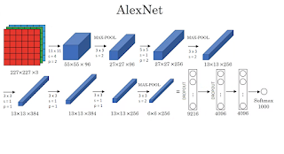
Do you wonder about how to come up with different design choices (architecture, optimization method, data manipulation, loss function, etc.) for the deep learning model so that it gives the best performance? Let's look at the different CNN architectures that have performed well in the past on image classification tasks. The ImageNet Large Scale Visual Recognition Challenge (ILSVRC) was the huge benchmark for image classification because it held a yearly challenge from 2010 to 2017 where teams around the world would compete with their best-performing classification models. This competition uses a subset of ImageNet's images containing 1.2 million high-resolution images with 1000 different classes and challenges researchers to achieve the lowest top-1 and top-5 error rates (top-5 error rate would be the percent of test images where the correct label is not one of the model's five most likely labels). For the first two years (2010 and 2011), the winning systems were...

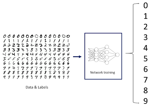
Image classification is a fundamental task in computer vision that attempts to comprehend an entire image as a whole. The goal is to classify the image by assigning it to a specific class label. Typically, image classification refers to images in which only one object appears and is analyzed. Now that we have all the ingredients required to code up our deep learning architecture, let's dive right into creating a model that can classify handwritten digits (MNIST Dataset) using Convolutional Neural Networks from scratch. The MNIST dataset consists of 70,000 $28 \times 28$ black-and-white images of handwritten digits. I will be using Pytorch for this implementation. Don't forget to change the runtime to GPU to get accelerated processing! The first step is to import the relevant libraries that we will be using throughout our code. import torch from torch import nn import torchvision import matplotlib.pyplot as plt Downloading and Pre-processing the Dataset The dataset ...

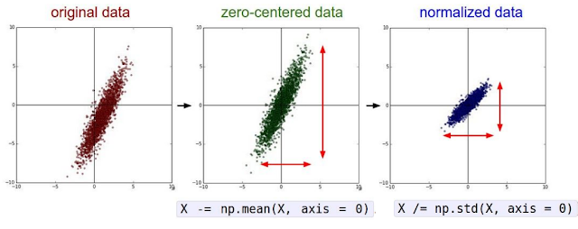
In the previous post, we talked about Convolution and Pooling layers. Stacking a large number of these layers (CNNs with activation functions and pooling) results in a Deep CNN architecture, which is often hard to train. It becomes very difficult to converge once they become very deep. The most common solution to this problem is Batch Normalization . The idea is to normalize the outputs of a layer so that they have zero mean and unit variance. If you ask why?. The distribution of the inputs to layers deep in the network may change after each mini-batch when the weights are updated. This can cause the learning algorithm to forever chase a moving target. This change in the distribution of inputs to layers in the network is referred to as the technical name " internal covariate shift " and batch normalization helps to reduce this internal covariance shift, improving optimization. We introduce batch normalization as a layer in our network that takes in inputs and normalizes...

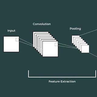
Linear Neural Networks that we have talked about till this point do not work when dealing with image data, as they don't respect the spatial structure of images. When a neural network is applied to a 2D image, it flattens it out in 1D and then uses it as input. This creates a need for a new computational node that operates on images - Convolutional Neural Networks (CNNs). A convolution layer has a 3D image tensor (3 X H X W) as an input and a 3D filter (also called a kernel) that convolves over the image, i.e. slides over the image spatially, computing dot products. It should be noted that since it a 2D operation, the number of depth channels (here its 3 RGB) always has to match the number of depth channels in the filter. The figure below shows an example of the convolution operation. The values in the filter are the weights that are learned from training, and the same filter gets applied over all the positions of the image. Here is what it would look like in 3D. ...

Datasets drive our choices for all the deep learning hyperparameters and peculiarities involved in making accurate predictions. We split the dataset into a training set, test set, and validation set. Our model is trained on the training set, and we choose the hyperparameters (usually by trial and error) on the validation set. We select the hyperparameters that have the highest accuracy on the validation set and then fix our model. The test set is reserved to be used only once at the very end of our pipeline to evaluate our model. Our algorithm is run exactly once on the test set and that accuracy gives us a proper estimate of our model's performance on truly unseen data. Now that we have created our training set to perform the optimization process, let's look at how manipulating this data can help us train our model. Data Preprocessing The loss function is computed on the mini-batch of the training data at every step of the optimization algorithm. Therefore, the loss ...

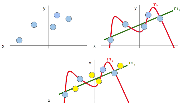
Our motivation behind using optimization was to obtain that specific set of weights that incurs the least loss on our training data to achieve the maximum possible accuracy on the test set. But this never works in practice! (yes, you read that right). If we are trying to incur the least loss on the training data, i.e., fit the training data perfectly (called overfitting), our model might not always fit the test data perfectly. It is important to remember that the training and the test set are assumed to be sampled from a common dataset, and our aim is to ensure that our model fits this dataset. To achieve good accuracy, we must ensure that our model generalizes well to fit the test set as much as possible. We apply this in practice using a technique called regularization. Let's understand this concept with a simple example. The blue points are the training data, and we fit two different models, m1 (polynomial) and m2 (linear). While m1 perfectly fits the training set (overfits...

All the variants of gradient descent, such as Momentum, Adagrad, RMSProp, and Adam, use a learning rate as a hyperparameter for global minimum search. Different learning rates produce different learning behaviors (refer to the Figure below), so it is essential to set a good learning rate, and we prefer to choose the red one. But it is not always possible to come up with one "perfect" learning rate by trial and error. So what if don't keep the learning rate fixed, and change it during the training process? We can choose a high learning rate to allow our optimization to make quick progress in the initial iterations of training and then decay it over time. This would speed up our algorithm and result in better performance characteristics. This mechanism of changing the learning rates over the training process is called learning rate schedules. Let's see some commonly used learning rate schedulers, Step schedule - We start with a high learning rate (like the g...