YA's Blog

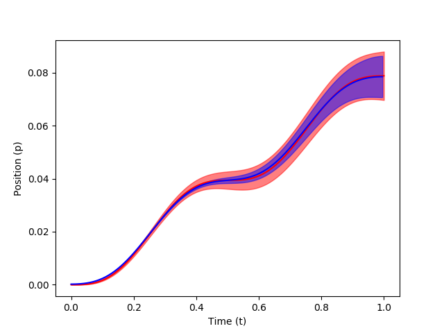
The modulation of via-points, final positions, and velocities is carried out using conditioning so that MP can adapt to new situations. In order to condition the MP to reach a certain state $y^*$ at any time point $t$, a desired observation $x^*_t = [y_t^*, \Sigma_y^*]$ is added to the model. Applying Bayes theorem, \begin{equation} p(w|x^*_t) \propto \mathcal{N} (y^*_t | \Psi_t w, \Sigma^*_y) \; p(w) \end{equation} where state vector $y^*_t$ defines the desired position and velocity at a time $t$ and $\Sigma_y^*$ defines the accuracy of the desired observation. The conditional distribution $p(w|x^*_t)$ is Gaussian for a Gaussian trajectory distribution, whose mean and variance are given by, \begin{equation} \mu_w^{[new]} = \mu_w + L (y_t^* - \Psi_t^T \mu_w), \hspace{10mm} \Sigma_w^{[new]} = \Sigma_w - L \Psi_t^T \Sigma_w, \end{equation} where $L = \Sigma_w \Psi_t {(\Sigma_y^* + \Psi_t^T \Sigma_w \Psi_t)}^{-1}$. Let's code via_points = [(0.2, .02),

In this post, we describe how a Probabilistic Movement Primitive can be learnt from demonstrations using supervised learning. Learning from Demonstrations To simplify the learning of the parameters $\theta$, a Gaussian is assumed for $p(w; \theta) = \mathcal{N}(w | \mu_w, \Sigma_w)$ over $w$. The distribution $p(y_t| \theta)$ for time step $t$ is written as, \begin{equation} \begin{aligned} p(y_t| \theta) & = \int p(y_t| w) \; p(w; \theta) dw, \\ & = \int \mathcal{N}(y_t | \Phi_t w, \Sigma_y) \; \mathcal{N}(w | \mu_w, \Sigma_w), \\ & = \mathcal{N}(y_t | \Phi_t \mu_w, \Psi_t \Sigma_w \Phi_t^T + \Sigma_y). \end{aligned} \end{equation} It can be observed from the above equation, that the learnt ProMP distribution is Gaussian with, \begin{equation} \mu_t = \Phi_t \mu_w, \hspace{10mm} \Sigma_t = \Phi_t \Sigma_w \Phi_t^T + \Sigma_y \end{equation} Learning Stroke-based Movements For stroke-based movements, the parameter $\theta = \{ \m

As a continuation of our series on ProMPs, we will introduce the concepts of phase variable and basis functions in this post. Temporal Modulation The execution speed of the movement can be adjusted with temporal modulation. A phase variable $z$ is introduced (similar to the DMP approach) to separate the movement from the time signal. We can vary the speed of the movement by regulating the rate of phase variable. The phase is defined as $z_0 = 0$ at the start of the movement and $z_T = 1$ at the end (so as to normalize it). Phase defines how quickly the time evolves for a trajectory. The basis function $\phi(t)$ now directly depend on the phase instead of time, \begin{equation} \phi_t = \phi(z_t), \; \; \; \dot{\phi}_t = \dot{\phi}(z_t) \dot{z}_t. \label{eq12} \end{equation} Let's code We choose a monotonically increasing function with time that starts at 0 and ends at 1. By default, the phase speed is taken as 1. def get_phase_variables(phase_speed): phase_star

In the previous post, we talked about Dynamic Movement Primitive (DMP) framework. While DMP is an attractive MP architecture for generating stroke-based and rhythmic movements, it is a deterministic approach that can only represent the mean solution, which is known to be suboptimal. This creates a need for a more sophisticated MP architecture that not can not only overcome these problems but can also exhibit various useful properties like conditioning of trajectories and adaptation to new situations. Probabilistic Movement Primitives (ProMPs) is the only existing approach that exhibits many such properties in one unified framework. In this ProMP series, we will be talking about the theory behind this framework and simultaneously code each part of this framework in Python. Probabilistic Movement Primitives is a probabilistic formulation of MPs that maintains a distribution over trajectories. Such a distribution over trajectories automatically encodes the variance of the movements,

Robot manipulation and motion planning often take place in continuous state-action space where the objective is to define a desired trajectory that reaches a particular goal state. Movement Primitives (MPs) is a well established approach that formalizes the the learning of coordinated movements from Learning from Demonstrations (LfD). One primitive creates a family of movements that all converge to the same goal called a attactor point, which solves the problem of generalization. Dynamic Movement Primitives (DMPs) are learnable non-linear attractor systems that can produce both discrete as well as repeating trajectories. The theory behind DMPs is well described in this post. Consider a spring damper system shown below. General motion equation of this system can be written as: $\ddot{x} = K^p [y - x] - K^v \dot{x}$, where $K^p$ is the spring constant and $K^V$ damps the system. A spring-damper system is used because of its ability to converge to the goal state after excitation in