Regularization: Weight decay, Dropout, Early stopping
Our motivation behind using optimization was to obtain that specific set of weights that incurs the least loss on our training data to achieve the maximum possible accuracy on the test set. But this never works in practice! (yes, you read that right). If we are trying to incur the least loss on the training data, i.e., fit the training data perfectly (called overfitting), our model might not always fit the test data perfectly. It is important to remember that the training and the test set are assumed to be sampled from a common dataset, and our aim is to ensure that our model fits this dataset. To achieve good accuracy, we must ensure that our model generalizes well to fit the test set as much as possible. We apply this in practice using a technique called regularization.
Let's understand this concept with a simple example. The blue points are the training data, and we fit two different models, m1 (polynomial) and m2 (linear). While m1 perfectly fits the training set (overfits!), m2 generalizes the data. Look at the third image, where the yellow points are the test set. Clearly, m2 would perform better than m1. We use regularization to make sure we choose simpler models (generalize more) and prevent the model from overfitting.

Weight decay
In this type of regularization, we prevent overfitting by zeroing out some weights of our model. An additional term is added in computation of loss over the training data as, \begin{align*} L &= \frac{1}{N} \sum_{i = 1}^N L_i(x_i, y_i, W) + \lambda R(W) \end{align*} where $\lambda$ is the hyperparameter that controls the regularization strength. Since we minimize this loss function in our optimization process, the added term decays some weights of our model. $R(W)$ for different types of weight decay can be written as, \begin{align*} \text{L2: } & R(W) = \sum_k \sum_l W_{k,l}^2 \\ \text{L1: } & R(W) = \sum_k \sum_l |W_{k,l}| \\ \text{Elastic Net (L1 + L2) : } & R(W) = \sum_k \sum_l \beta W_{k,l}^2 + |W_{k,l}| \\ \end{align*} L2 regularization shrinks weights proportionally to its size, so bigger weights gets shrunk more (since we are adding the square of them in the loss function). Whereas L1 regularization shrinks all the weights by the same amount, with the smaller weights getting zeroed out.
L2 regularization (also called weight decay) is the most commonly used and can directly be added in our optimizer instance of Pytorch as $\lambda$ = 1e-4
optimizer = torch.optim.SGD(model.parameters(), lr=1e-3, weight_decay=1e-4)Dropout
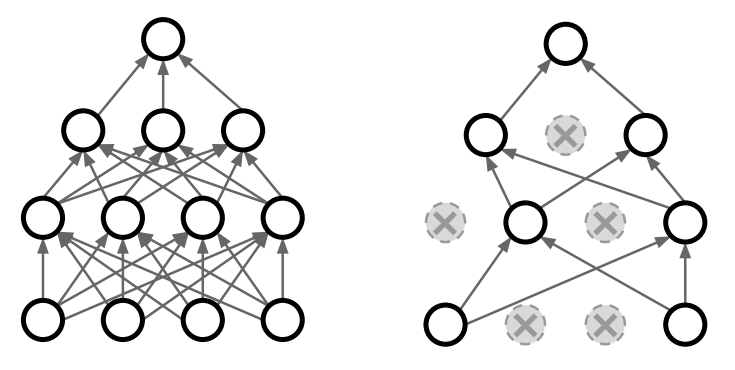
In the forward pass, we randomly set some of the neurons to zero, as shown in the figure below. The probability of dropping is a hyperparameter and is usually set to 0.5.
Since we are randomly zeroing out neurons in each layer of our network in each forward pass, we would obtain outputs that are also random. We need to average out this randomness at test time to have a deterministic output. So, if we are randomly removing half of the nodes in the forward pass (p=0.5), then for testing, we would use the full network but shrink the outputs by half (multiply by dropout probability). A derivation of the same is shown below for a single neuron.

By doing this, we scale the activations so that for each neuron: output at test time = expected output at training time (average out the randomness). Having two different behaviors of our model at training and test time looks cumbersome, so in practice, we use a variant called inverted dropout. In the forward pass, we randomly mask half of the neurons and double the output of the remaining neurons, so we don't have to change anything at the test time.
Introducing randomness in our network helps the model generalize better and prevent overfitting. Furthermore, it helps our optimizer to jump out of local minima by stimulating dead neurons during the training process. Another interpretation of dropouts is training a large ensemble of sub-networks that share weights.
Dropout can directly be implemented in Pytorch when defining our model as,
model = torch.nn.Sequential(torch.nn.Linear(3072, 100),
	torch.nn.ReLU(),
	torch.nn.Dropout(p=0.5),
    	torch.nn.Linear(100, 10))
Early Stopping
This notion of early stopping helps us to choose the num_steps hyperparameter, i.e., how long should we train our model? When training, we look at three curves: training loss as a function of iterations (should be decaying exponentially) and training and validation accuracy as a function of iterations. These curves give some sense of the health of our network.

Early stopping is a fairly simple regularization technique, where we stop the training process when the validation accuracy decreases. Training further would increase training accuracy (as our model starts to overfit), but it would perform very poorly on our test set (as the validation set is a good representation of the test set).


Comments
Post a Comment