AlexNet: The First CNN to win ImageNet Challenge

Do you wonder about how to come up with different design choices (architecture, optimization method, data manipulation, loss function, etc.) for the deep learning model so that it gives the best performance? Let's look at the different CNN architectures that have performed well in the past on image classification tasks.

The ImageNet Large Scale Visual Recognition Challenge (ILSVRC) was the huge benchmark for image classification because it held a yearly challenge from 2010 to 2017 where teams around the world would compete with their best-performing classification models. This competition uses a subset of ImageNet's images containing 1.2 million high-resolution images with 1000 different classes and challenges researchers to achieve the lowest top-1 and top-5 error rates (top-5 error rate would be the percent of test images where the correct label is not one of the model's five most likely labels).

For the first two years (2010 and 2011), the winning systems were not neural network-based at all. They used multiple layers of hand-designed feature extractors with linear neural networks on top.

Training CNNs were prohibitively expensive to apply on large scale to high-resolution images during that time. It was in 2012 with the introduction of GPUs paired with a highly-optimized implementation of 2D convolutions and the ImageNet dataset containing enough labeled examples, it became easy to train such models without severe overfitting.

AlexNet was the largest convolutional neural network trained at that time and achieved the best results ever reported on the ImageNet dataset, crushing all the other competitors by a big margin. This made CNNs a mainstream topic in the field of computer vision and AlexNet can undoubtedly be called one of the most influential research works in this field (the number of citations this paper has is just crazy!).

Data Manipulation: Since the images of the dataset are of variable size, they are first downsampled to a fixed size of 256 $\times$ 256. This is done by rescaling the shortest side of a rectangular image to a length of 256 and then cropping out the central 256 $\times$ 256 patches. The mean image is then subtracted from the training set.

Two forms of data augmentation techniques are applied to the training data to reduce overfitting, which is performed on the fly on the CPU while the GPUs train the previous batch of data, so essentially is computationally free.

1. The first form consists of extracting random 224 $\times$ 224 patches (and their horizontal reflections) from the original image, increasing the size of the training set by a factor of 2048. At test time, the network makes a prediction by extracting five 224 $\times$ 224 patches (the four corner patches and the center patch) as well as their horizontal reflections (ten patches in total), and averaging the predictions on them.
   
   
   
   
   
2. The second form is called PCA Color Augmentation (also called Fancy PCA) which consists of altering the intensities of the RGB channels in the training images. More details about this method and the code to implement it can be found here: Fancy PCA. This scheme approximately captures an important property of images that object identity is invariant to changes in the intensity and color of the illumination and reduces the top-1 error rate by over 1%.

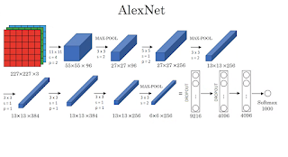
Architecture: The model has 8 layers: 5 Convolution Layers and 3 Fully-connected layers. The authors mention that this depth is vital as it was found that removing any convolution layer resulted in inferior performance. The output of the last fully-connected layer is fed to a 1000-way softmax (which produces a distribution over the 1000 class labels).

The original paper mentions an input image shape of 224 $\times$ 224 and uses a pad of 3 in the first convolution. In practice, we begin with an image of size 227 $\times$ 227, and the padding is made zero, so as to encompass more information from the image (as padding of zero has no information)

Tanh non-linearity was commonly used during that time, and AlexNet was the first CNN architecture that used ReLU (called it non-saturating nonlinearity). The authors argued that CNNs train several times faster with ReLU than their equivalent tanh units because tanh saturates for large absolute values of activations killing the gradient (vanishing gradient problem). Today, ReLU is the default choice of the activation function.

Max-pooling layers are included in the network with a kernel size of 3 and stride of 2, and they call it "overlapping pooling". Compared to local pooling (kernel size = 2 and stride = 2), overlapping pooling reduces the top-1 and top-5 error rates by 0.4% and 0.3% respectively because they are slightly more difficult to overfit.

Dropout layers with a probability of 0.5 are also added in the first two fully-connected layers to prevent overfitting during training. Without dropout, the network exhibits substantial overfitting. It roughly doubles the number of iterations required to converge.

AlexNet uses "Local Response Normalization" that reduces top-1 and top-5 error rates by 1.4% and 1.2% respectively. This is not used anymore so we won't talk about it, but it was an early precursor to batch normalization.

Training: The model was trained on the Cross-entropy loss function using stochastic gradient descent with a batch size of 128 examples, momentum of 0.9, and weight decay of 0.0005. It was found that this small amount of weight decay was important for the model to learn as it is not merely a regularizer, but it also reduces the model's training error.

The weights for each layer were initialized from a zero-mean Gaussian distribution with a standard deviation of 0.01. The biases in the second, fourth, and fifth convolutional layers, as well as in the fully-connected layers, are initialized with the constant 1 and for the remaining layers with the constant 0.

An equal learning rate is used for all the layers. The learning rate was initialized at 0.01 and reduced three times prior to termination, which was divided by 10 when the validation error rate stopped improving with the current learning rate.

Above is a typical AlexNet architecture image that you would see almost everywhere. The model was spread across two GTX 580 3GB GPUs as the model was too big to fit on one GPU memory, and they communicated only in certain layers to save computation. However, we don't need such a complicated scheme anymore as we can train the entire model on a single GPU (Google colab provides 12GB/16GB GPUs today).

It took about 90 epochs through the training set of 1.2 million images, which took five to six days on these two GPUs.

Overall AlexNet showed the power of the convolutional neural network in achieving record-breaking results on an image classification task. Important design choices of the paper are,

• 8 Layers: 5 CNN layers + 3 Fully-connected layers
• Activation Function: ReLU
• Data pre-processing: subtract mean image
• Heavy data augmentation
• Regularization: L2 Weight decay ($\lambda$ = 5e-4), Dropout (p=0.5)
• Learning rate: 0.01 and reduced (divided by 10) when val accuracy plateaus
• Optimization Method: SGD + Momentum (m=0.9) with batch size of 128
• Loss function: Cross-Entropy loss

Link to the Paper: ImageNet Classification with Deep Convolutional Neural Networks