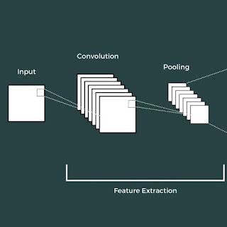
Neural Network for Images: Convolutional Neural Networks (CNNs)

Linear Neural Networks that we have talked about till this point do not work when dealing with image data, as they don't respect the spatial structure of images. When a neural network is applied to a 2D image, it flattens it out in 1D and then uses it as input. This creates a need for a new computational node that operates on images - Convolutional Neural Networks (CNNs).

A convolution layer has a 3D image tensor (3 X H X W) as an input and a 3D filter (also called a kernel) that convolves over the image, i.e. slides over the image spatially, computing dot products. It should be noted that since it a 2D operation, the number of depth channels (here its 3 RGB) always has to match the number of depth channels in the filter. The figure below shows an example of the convolution operation.

The values in the filter are the weights that are learned from training, and the same filter gets applied over all the positions of the image. Here is what it would look like in 3D.

Each 3D filter gives a 2D output called an activation map. Having only one filter does not make much sense, so a convolution layer involves convolving the input with a bank of filters (different filters with different weight values). When we convolve these filters with the input, we get one 2D activation map for each filter. We stack all the 2D activation maps together to obtain a 3D output tensor with the number of depth channels equal to the number of filters in that layer. An example is shown below,

As you can clearly note that the size of the activation map is not equal to the size of the image (or the input). Actually, it depends on the size of the filter. Here's how, \begin{align*} \underbrace{N \times C_{in} \times H \times W}_{\text{Input size}} + \underbrace{C_{out} \times C_{in} \times K_w \times K_h}_{\text{Filters size}} \Rightarrow \underbrace{N \times C_{out} \times H' \times W'}_{\text{Output size}} \end{align*} where $N$ is the number of images in a single mini-batch, $C_{in}$ is the number of input channels and $C_{out}$ is the number of output channels or the number of filters in that convolution layer. Usually, $H = W$ (considering a square image) and $K_w = K_h = K$ (considering a square kernel), the output size $H' = W'$ is given by, \begin{align*} W' = \frac{(W - K + 2P)}{S} + 1 \end{align*} where $P$ is the padding size and $S$ is the stride. Padding is a process of adding zeros around the input, applied so that the input size does not shrink after convolution operation. Stride is often used to downsample our input, where we modify the amount of movement of the filter over the input. So in a stride of 2, rather than placing our filter on every pixel of the image, we would place it on alternate pixels.

Just like linear networks, stacking multiple convolution layers would result in one single big convolution. So, we need to have activations after each convolution. We even sometimes have $1 \times 1$ convolution layer which gives MLP operating on each input pixel separately. Common choices:

• $P = (K-1)/2 \hspace{1mm}$ gives "same" padding (output size = input size)
• $C_{in}$, $C_{out}$ = 32, 64, 128, 256 (in Powers of 2)
• K = 3, P = 1, S = 1 (Kernel = $3 \times 3$)
• K = 5, P = 2, S = 1 (Kernel = $5 \times 5$)
• K = 1, P = 0, S = 1 (Kernel = $1 \times 1$)
• K = 3, P = 1, S = 2 (Downsample by 2)

Pooling layers are another way (and much more preferred) to downsample a large input. The concept of the filter is the same as the convolution layer but instead of convolving, we take the maximum value of the elements in a kernel. Such a type of operation is called max-pooling and it takes only the kernel size and stride as hyperparameters. An example is shown below where the kernel size is 2 and the stride is 2.

Another common pooling operation is average pooling, where we take the average of all the elements in the kernel. Pooling layers do not have any learnable parameters so, during backpropagation, it simply points to the value that had maximum in the previous layer (where the value came from). It itself introduces non-linearity to our model, so any kind of activation is not required after pooling layers.

It also introduces translational invariance to our input, which means if a cat feature is present in the top-left corner of the filter or in the right-bottom, it will still give the same output as we are essentially performing the max over the kernel. The output remains the same even if the exact position of something in the image changes a little.

It should be noted that when we downsample our input using pooling or strided convolutions, the number of channels increases so that the total volume remains preserved.