Using Learning Rate Schedules for Training

All the variants of gradient descent, such as Momentum, Adagrad, RMSProp, and Adam, use a learning rate as a hyperparameter for global minimum search. Different learning rates produce different learning behaviors (refer to the Figure below), so it is essential to set a good learning rate, and we prefer to choose the red one.

But it is not always possible to come up with one "perfect" learning rate by trial and error. So what if don't keep the learning rate fixed, and change it during the training process?

We can choose a high learning rate to allow our optimization to make quick progress in the initial iterations of training and then decay it over time. This would speed up our algorithm and result in better performance characteristics. This mechanism of changing the learning rates over the training process is called learning rate schedules. Let's see some commonly used learning rate schedulers,

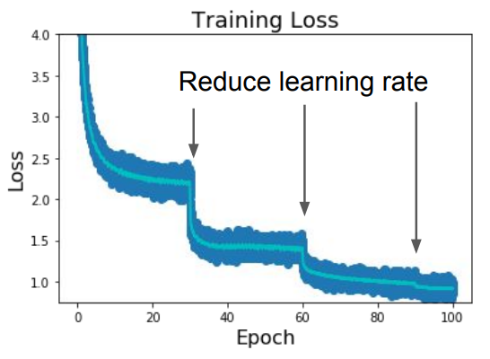
Step schedule - We start with a high learning rate (like the green one). When the curve starts flattening, we reduce the learning rate and continue the same process until convergence. E.g., for ResNets, multiplying LR by 0.1 after epochs 30, 60, and 90 would result in a learning curve as shown beside. But this kind of scheduling introduces a lot of new hyperparameters - at what fixed points should we decay the LR, and to what value? Tuning them usually takes a lot of time.

Decay functions - Instead of explicitly choosing fixed time points, we use a function that determines the learning rate at each epoch, hence it has no additional hyperparameters. We start with some initial learning rate and then decay it over the training process with a function to zero.

Cosine scheduling uses a cosine function. It is a very popularly used learning rate scheduler in computer vision problems. We can also linearly decay the learning rate over time. Such kind of scheduling is used commonly for language tasks. The Transformers paper (Attention is all you need) used an inverse square root decay function. The learning rate at epoch $t$ in each of these cases is given as, \begin{align*} \text{Cosine: } & \eta_t = \frac{\eta_0}{2} ( 1 + cos \frac{t \pi}{T}) \\ \text{Linear: } & \eta_t = \eta_0 (1 - \frac{t}{T}) \\ \text{Inverse Sqrt: } & \eta_t = \frac{\eta_0}{ \sqrt{t} }\\ \end{align*} where $\eta_0$ is the initial learning rate and $T$ is the total number of epochs.

LR schedules are an optional technique that can be implemented to boost learning. It is important to note that using LR schedules with SGD + Momentum is fairly important. Still, if we are using one of the more complicated optimization method, such as Adam, then it often works well even with a constant learning rate. In fact, SGD + Momentum can outperform Adam but may require more tuning of LR and schedule.

Recall the training block code of the previous post. Pytorch's optim package can be used to implement these LR schedulers. After each epoch in the training loop, we use .step() function to update the learning rate as per our schedule.

model = torch.nn.Sequential(torch.nn.Linear(3072, 100),
	torch.nn.ReLU(),
        torch.nn.Linear(100, 10))
optimizer = torch.optim.SGD(model.parameters(), lr=initial_learning_rate)
scheduler = optim.lr_scheduler.CosineAnnealingLR(optimizer, num_steps)
mini_batches = torch.utils.data.DataLoader(data, batch_size=batch_size)
for t in range(num_steps):
  for X_batch, y_batch in mini_batches:
  	y_pred = model(X_batch)			
  	loss = loss_fn(y_pred, y_batch)
    	loss.backward()
  	optimizer.step()
  	optimizer.zero_grad()
  scheduler.step()