Image Classification using CNNs: MNIST dataset

Image classification is a fundamental task in computer vision that attempts to comprehend an entire image as a whole. The goal is to classify the image by assigning it to a specific class label. Typically, image classification refers to images in which only one object appears and is analyzed.

Now that we have all the ingredients required to code up our deep learning architecture, let's dive right into creating a model that can classify handwritten digits (MNIST Dataset) using Convolutional Neural Networks from scratch. The MNIST dataset consists of 70,000 $28 \times 28$ black-and-white images of handwritten digits. I will be using Pytorch for this implementation. Don't forget to change the runtime to GPU to get accelerated processing!

The first step is to import the relevant libraries that we will be using throughout our code.

import torch
from torch import nn
import torchvision
import matplotlib.pyplot as plt

Downloading and Pre-processing the Dataset

The dataset is downloaded into two subsets, the train set containing 60,000 images and the test set containing 10,000 images. While downloading, we apply some transformations to the images - convert them to tensors for processing them in the convolution layers and normalizing them. Each pixel value is originally [0,255] that gets divided by 255 while getting converted to tensor, resulting in a range [0,1]. We further normalize the image with a mean of 0.5 and a standard deviation of 0.5 to obtain the pixel values in the range [-1,1].

my_transform = torchvision.transforms.Compose([
        torchvision.transforms.ToTensor(),
        torchvision.transforms.Normalize((0.5,), (0.5,))
])

# Download the dataset
mnist_trainset = torchvision.datasets.MNIST(root='./data', train=True, download=True, transform=my_transform)
mnist_testset = torchvision.datasets.MNIST(root='./data', train=False, download=True, transform=my_transform)

Loading the Dataset

As we discussed in this post, the test set is reserved to be used only once at the very end of our pipeline to evaluate our model. We randomly split the training data into a training set containing 80% of the images and a validation set containing 20% of the images and then build their loaders. I have defined a batch size of 64 for both the loaders but it can be set in any power of 2 (why? check out mini-batch gradient descent).

# Split the dataset into train set(80%) and validation set(20%) and then load it
len_train = int(0.8 * len(mnist_trainset))
len_val = len(mnist_trainset) - len_train
train_dataset, val_dataset = torch.utils.data.random_split(mnist_trainset, [len_train, len_val])

# train_loader is the data loader containing the training samples
train_loader = torch.utils.data.DataLoader(train_dataset, batch_size = 64, shuffle = True)

# val_loader is the data loader containing the validation samples
val_loader = torch.utils.data.DataLoader(val_dataset, batch_size = 64, shuffle = True)

Defining the Architecture

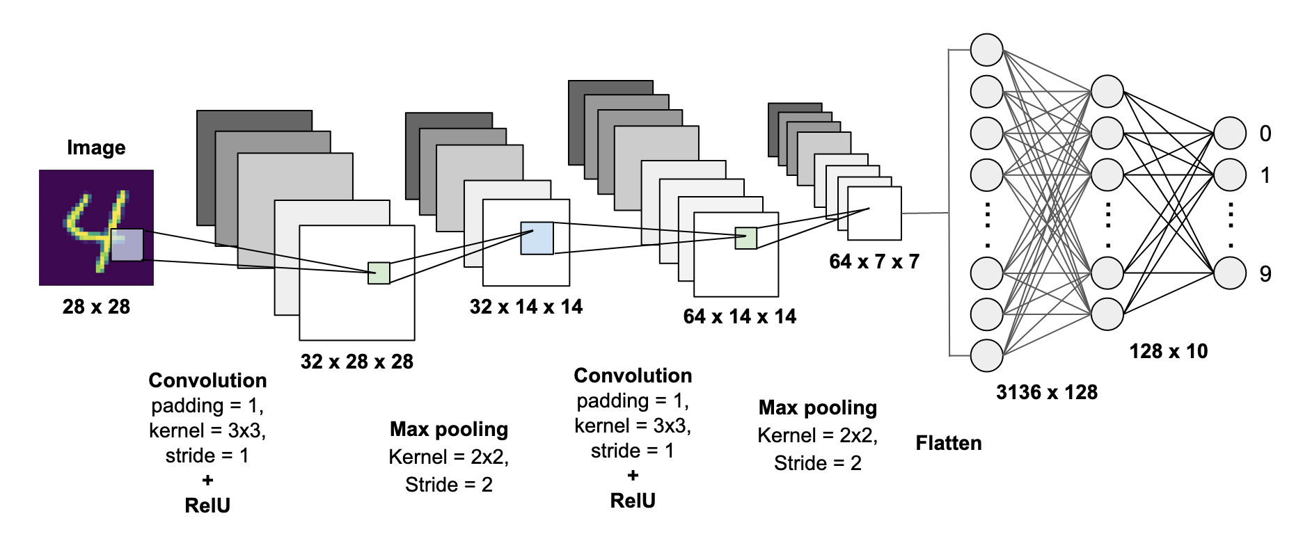
We will be using the Convolution Layer (link) to extract features from the images followed by Batch Norm (link) and Activation function (link). We add then add the Pooling layer (to downsample the images) and repeat this block again. Next, the features are flattened and fed into a fully-connected layer followed by an activation function. We then add a Dropout layer (link) for regularization, followed by another fully connected layer that gives 10 outputs (for 10 digits).

# CUDA for PyTorch
use_cuda = torch.cuda.is_available()
device = torch.device("cuda:0" if use_cuda else "cpu")

# Creating the architecture
class DigitClassification(torch.nn.Module):
    def __init__(self):
        super(DigitClassification, self).__init__()

        self.conv1 = torch.nn.Conv2d(in_channels=1, out_channels=32, kernel_size=3, stride=1, padding=1)
        self.bn1 = nn.BatchNorm2d(32)
        self.max_pool1 = torch.nn.MaxPool2d(kernel_size=2, stride=2)

        self.conv2 = torch.nn.Conv2d(in_channels=32, out_channels=64, kernel_size=3, stride=1, padding=1)
        self.bn2 = nn.BatchNorm2d(64)
        self.max_pool2 = torch.nn.MaxPool2d(kernel_size=2, stride=2)

        self.fc1 = torch.nn.Linear(7 * 7 * 64, 128)
        self.dropout = torch.nn.Dropout(p=0.5)
        self.fc2 = torch.nn.Linear(128, 10)

        self.relu = nn.ReLU()
        pass
        
        
    def forward(self, x):
        x = self.conv1(x)
        x = self.relu(self.bn1(x))
        x = self.max_pool1(x)

        x = self.conv2(x)
        x = self.relu(self.bn2(x))
        x = self.max_pool2(x)

        x = torch.flatten(x, 1)

        x = self.relu(self.fc1(x))
        x = self.dropout(x)
        x = self.fc2(x)

        return x

# Instantiating the network
model = DigitClassification().to(device)

Training our Model

Now that we have defined our model let's train it! I will be used the Adam optimizer and the Cross-entropy Loss function for learning the weights of our model. The training process is very similar to that defined in the post Implementing Backpropagation. Since we are using Batch Normalization that behaves differently during train and test times, we have to include model.train() and model.eval() to denote two different modes of our model while training and evaluating respectively.

We get the training loss for the entire epoch by adding all the losses for each batch iteration and averaging them. After that, we compare the model’s prediction with the actual labels and calculate the accuracy of the model.

num_epochs = 10

criterion = nn.CrossEntropyLoss()
learning_rate = 0.001
optimizer = torch.optim.Adam(model.parameters(), learning_rate)

train_loss, val_loss = [], []
train_acc, val_acc = [], []

for epoch in range(num_epochs):
  
  model.train()
  running_loss = 0.
  correct, total = 0, 0 
  for i, (image, label) in enumerate(train_loader):
    image = image.to(device)
    label = label.to(device)

    output = model.forward(image)
    optimizer.zero_grad()
    loss = criterion(output, label)
    loss.backward()
    optimizer.step()

    running_loss += loss.item()
    
    _, predicted = torch.max(output, dim=1)
    total += label.size(0)
    correct += (predicted == label).sum().item()

  train_loss.append(running_loss/len(train_loader))
  train_acc.append(correct/total)

  model.eval()
  running_loss = 0.
  correct, total = 0, 0 
  for i, (image, label) in enumerate(val_loader):
    image = image.to(device)
    label = label.to(device)

    output = model.forward(image)
    loss = criterion(output, label)

    running_loss += loss.item()
    
    _, predicted = torch.max(output, dim=1)
    total += label.size(0)
    correct += (predicted == label).sum().item()

  val_loss.append(running_loss/len(train_loader))
  val_acc.append(correct/total)

  print('\nEpoch: {}/{}, Train Loss: {:.4f}, Val Loss: {:.4f}, Val Accuracy: {:.4f}'.format(epoch + 1, num_epochs, train_loss[-1], val_loss[-1], val_acc[-1]))


plt.figure(1)
plt.plot(list(range(num_epochs)), train_loss, label='Training Loss')
plt.plot(list(range(num_epochs)), val_loss, label='Validation Loss')
plt.xlabel("Epochs")
plt.ylabel("Loss")
plt.title('Epoch vs Loss')
plt.legend()

plt.figure(2)
plt.plot(list(range(num_epochs)), train_acc, label='Training Accuracy')
plt.plot(list(range(num_epochs)), val_acc, label='Validation Accuracy')
plt.xlabel("Epochs")
plt.ylabel("Accuracy")
plt.title('Epoch vs Accuracy')
plt.legend()

plt.show()

After setting the model to eval mode, we iterate over each batch from the validation data loader using the enumerate function. We do similar steps as training but we do not backpropagate the loss. The plots generated from training look something like this.

Testing our Model

Just like we did for the training data, let's create a test loader first. I have kept the batch size as 1 because we aren't doing any kind of optimization here so batches are irrelevant.

test_loader = torch.utils.data.DataLoader(mnist_testset, batch_size = 1)

model.eval()
correct, total = 0, 0 
for i, (image, label) in enumerate(test_loader):
    image = image.to(device)
    label = label.to(device)

    output = model.forward(image)
    
    _, predicted = torch.max(output, 1)
    total += label.size(0)
    correct += (predicted == label).sum().item()

print(correct/total)

We enumerate through our test data loader and calculate the model's accuracy on unseen data the same way we did with the validation loop. With this model, I got $99.2%$ accuracy on the test set by training the model for just 10 epochs!