YA's Blog

Imagine being able to generate photorealistic 3D models of objects and scenes that can be viewed from any angle, with details so realistic that they are indistinguishable from reality. That's what the Neural Radiance Fields (NeRF) is capable of doing and much more. With more than 50 papers related to NeRFs in the CVPR 2022, it is one of the most influential papers of all time. Neural fields A neural field is a neural network that parametrizes a signal. In our case, this signal is either a single 3D scene or an object. It is important to note that a single network needs to be trained to encode (capture) a single scene . It is worth mentioning that, unlike standard machine learning, the objective is to overfit  the neural network to a particular scene. Essentially, neural fields embed the scene into the weights of the network. 3D scenes are usually stored in computer graphics using voxel grids or polygon meshes. However, voxels are costly to store and polygon meshes are lim

Introduced in 2014 by Goodfellow. et al , Generative Adversarial Networks (GANs) revolutionized the field of Generative modeling. They proposed a new framework that generated very realistic synthetic data trained through a minimax two-player game. With GANs, we don't explicitly learn the distribution of the data $p_{\text{data}}$, but we can still sample from it. Like VAEs, GANs also have two networks: a Generator and a Discriminator that are trained simultaneously. A latent variable is sampled from a prior $\mathbf{z} \sim p(\mathbf{z})$ and passed through the Generator to obtain a fake sample $\mathbf{x} = G(\mathbf{z})$. Then the discriminator performs an image classification task that takes in all samples and classifies it as real ($1$) or fake ($0$). These are trained together such that while competing with each other, they make each other stronger at the same time. To summarize, A discriminator $D$ estimates the probability of a given sample coming from the

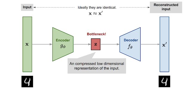
Till now, I have talked about supervised learning where our model is trained to learn a mapping function of data $\mathbf{x}$ to predict labels $\mathbf{y}$, for example, the tasks of classification, object detection, segmentation, image captioning, etc. However, supervised learning requires large datasets that are created with human annotations to train the models. The other side of machine learning is called unsupervised learning where we just have data $\mathbf{x}$, and the goal is to learn some hidden underlying structure of the data using a model. Through this approach, we aim to learn the distribution of the data $p(\mathbf{x})$ and then sample from it to generate new data, in our case images. Autoencoders An autoencoder is a bottleneck structure that extracts features $\mathbf{z}$ from the input images $\mathbf{x}$ and uses them to reconstruct the original data $\mathbf{x}'$, learning an identity mapping. Encoder: network that compresses the input into a latent-s

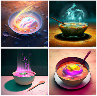
Diffusion models are a new class of state-of-the-art generative models that generate diverse high-resolution images. There are already a bunch of different diffusion models that include Open AI’s DALL-E 2 and GLIDE, Google’s Imagen, and Stability AI’s Stable Diffusion. In this blog post, we will dig our way up from the basic principles described in the most prominent one, which is the Denoising Diffusion Probabilistic Models (DDPM) as initialized by Sohl-Dickstein et al in 2015 and then improved by Ho. et al in 2020. Images produced by Dall-E 2 The basic idea behind diffusion models is rather simple. It takes an input image $\mathbf{x}_0$ and gradually adds Gaussian noise to it through a series of $T$ time steps. We will call this the forward process. A network is then trained to recover the original image by reversing the noising process. By being able to model the reverse process, we can start from random noise and denoise it step-by-step to generate new data. Forward Diffus

In 2015, Batch Normalization was discovered, which heralded the progress of architectures as it was now possible to train deep networks without using any tricks - allowing us to use much higher learning rates and be less careful about initialization. It also acts as a regularizer, eliminating the need for Dropout. Another major problem with deep networks was of vanishing/exploding gradients, but it was now being handled by Kaiming Initialization. With the stage set in place, experiments began on training deeper models. It was noted that when deeper networks are able to start converging, a degradation problem occurs: as we increase the depth, the accuracy gets saturated (which might be unsurprising) and then degrades rapidly. Unexpectedly, such degradation is not caused by overfitting (which was the initial guess), because adding more layers to a suitably deep model lead to higher training error. It turns out, deeper networks are underfitting ! By intuition, it is expect

The 2014 winner of the ImageNet challenge was the InceptionNet or GoogLeNet architecture from Google. The most straightforward way of improving the performance of deep neural networks is by increasing their size: depth (the number of layers) and width (the number of units at each layer). But with such a big network comes a large number of parameters (which makes it prone to overfitting) and increased use of computation resources. In order to cater to these problems, the design choices of GoogLeNet were focused on efficiency. Architecture: In order to very aggressively downsample the spatial dimensions of the input image at the beginning, GoogLeNet uses a Stem Network. This looks very similar to AlexNet or ZFNet (and local response normalization is used in this network). It then includes an Inception module, a local structure with parallel branches that was repeated many times throughout the entire network (just like stages in VGGNet). In order to eliminate the

With the advent of AlexNet, all the submissions to the ImageNet Large Scale Visual Recognition Challenge (ILSVRC) switched over to using convolutional neural networks. In 2013, the winner of this challenge was ZFNet, a modified version of AlexNet which gave better accuracy. It was also an 8-layer network that tweaked some of the layer configurations of AlexNet by trial and error. ZFNet used 7 $\times$ 7 sized filters in the first layer with a stride of 2 instead of 11 $\times$ 11 filters with a stride of 4. The intuition behind this is that we were losing a lot of pixel information (aggressively downsampling the input), which can be retained by having smaller filter sizes and small strides. The padding is removed for the first two conv layers (to match the subsequent conv layers shapes of AlexNet). With just these two changes, they are able to achieve a reasonably large increase in performance over AlexNet. AlexNet or ZFNet were designed in somewhat an ad-hoc manner with s