YA's Blog

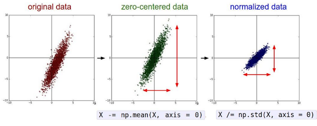
Datasets drive our choices for all the deep learning hyperparameters and peculiarities involved in making accurate predictions. We split the dataset into a training set, test set, and validation set. Our model is trained on the training set, and we choose the hyperparameters (usually by trial and error) on the validation set. We select the hyperparameters that have the highest accuracy on the validation set and then fix our model. The test set is reserved to be used only once at the very end of our pipeline to evaluate our model. Our algorithm is run exactly once on the test set and that accuracy gives us a proper estimate of our model's performance on truly unseen data. Now that we have created our training set to perform the optimization process, let's look at how manipulating this data can help us train our model. Data Preprocessing The loss function is computed on the mini-batch of the training data at every step of the optimization algorithm. Therefore, the loss

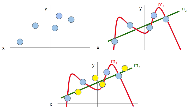
Our motivation behind using optimization was to obtain that specific set of weights that incurs the least loss on our training data to achieve the maximum possible accuracy on the test set. But this never works in practice! (yes, you read that right). If we are trying to incur the least loss on the training data, i.e., fit the training data perfectly (called overfitting), our model might not always fit the test data perfectly. It is important to remember that the training and the test set are assumed to be sampled from a common dataset, and our aim is to ensure that our model fits this dataset. To achieve good accuracy, we must ensure that our model generalizes well to fit the test set as much as possible. We apply this in practice using a technique called regularization. Let's understand this concept with a simple example. The blue points are the training data, and we fit two different models, m1 (polynomial) and m2 (linear). While m1 perfectly fits the training set (overfits

All the variants of gradient descent, such as Momentum, Adagrad, RMSProp, and Adam, use a learning rate as a hyperparameter for global minimum search. Different learning rates produce different learning behaviors (refer to the Figure below), so it is essential to set a good learning rate, and we prefer to choose the red one. But it is not always possible to come up with one "perfect" learning rate by trial and error. So what if don't keep the learning rate fixed, and change it during the training process? We can choose a high learning rate to allow our optimization to make quick progress in the initial iterations of training and then decay it over time. This would speed up our algorithm and result in better performance characteristics. This mechanism of changing the learning rates over the training process is called learning rate schedules. Let's see some commonly used learning rate schedulers, Step schedule - We start with a high learning rate (like the g

While we have talked about how optimization algorithms use the negative gradient of the loss function with respect to the weights to update the parameters of our model, we will now focus on how to actually compute these gradients on an arbitrary loss function. We use a backpropagation technique that creates a computation graph to perform a forward and backward pass on the model. In the forward pass, we compute outputs of each layer of our neural network sequentially. In the backward pass, we apply the chain rule for computing derivatives of each individual layer backward. Consider the example of a computation graph shown below. First we perform a forward pass where we have the value of inputs $x = -2, y = 5, z = -4$, \begin{align*} q &= x + y = -2 + 5 = -3\\ f & = z * q = -4 * -3 = -12 \end{align*} Now lets compute the backward pass, \begin{align*} & \frac{df}{df} = 1, \hspace{5mm} \frac{df}{dq} = z = -4, \hspace{5mm} \frac{df}{dz} = q = -3 \\ & \frac{d

In this post, we will make choices for components of our deep neural network architecture, including activation functions and how the weights of each layer get initialized to ease the optimization process.  A neural network is composed of interconnected layers, with every neuron in one layer connecting to every neuron in the next layer. Such a fully connected neural network is often called Multi-layer Perceptron (MLP). Let's dive right into defining our deep neural network architecture. \begin{align*} \text{Linear function: } & f = W x \\ \text{2-Layer Neural Network: } & f = W_2 \hspace{2mm} z(W_1 x) \\ \text{3-Layer Neural Network: } & f = W_3 \hspace{2mm} z_2(W_2 \hspace{2mm} z_1(W_1 x)) \\ \end{align*} The weights $W$ have 1s appended at the last column for the bias (called the bias trick). A typical deep learning model has many layers. The number of learnable weights is equal to the number of layers in the DNN (as each layer has an associated weigh

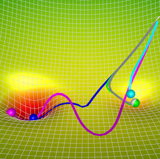
The loss function tells us how good our current classifier (with our current weights) is. Since we are a greedy bunch of people, we want to find those specific sets of weights that incurs a minimal loss on our training dataset to fit the data as well as we can to achieve the maximum possible accuracy on the test set. We generally initialize our model with some weights and then optimize them to obtain the best model. Optimization is the process of finding the set of parameters that minimize the loss function. Consider a landscape with (x,y) position as the weights and the height as the loss function. Our aim is to reach the bottom-most point of this landscape to obtain the weights that give the least loss. Since we do not have the exact equation of the landscape to compute the minima of the curve (not a convex optimization problem), we take small steps towards the direction of this minimum. The direction of the local steepest descent is nothing but the negative gradient of the loss