Optimization Methods: SGD, Momentum, AdaGrad, RMSProp, Adam

The loss function tells us how good our current classifier (with our current weights) is. Since we are a greedy bunch of people, we want to find those specific sets of weights that incurs a minimal loss on our training dataset to fit the data as well as we can to achieve the maximum possible accuracy on the test set. We generally initialize our model with some weights and then optimize them to obtain the best model. Optimization is the process of finding the set of parameters that minimize the loss function.

Consider a landscape with (x,y) position as the weights and the height as the loss function. Our aim is to reach the bottom-most point of this landscape to obtain the weights that give the least loss. Since we do not have the exact equation of the landscape to compute the minima of the curve (not a convex optimization problem), we take small steps towards the direction of this minimum. The direction of the local steepest descent is nothing but the negative gradient of the loss function with respect to the weights.

Gradient Descent

It is one of the most basic optimization algorithms where we iteratively take small steps (the size of the step is determined by the learning rate) in the direction of the negative gradient. A higher learning rate means taking larger steps toward the negative gradient, hoping that our algorithm would converge faster, but this often leads to unstable behavior. Lower learning rates are stable but take a lot of time to converge. Therefore it is very crucial to select an optimal learning rate. Its vanilla version looks as follows:

# Vanilla Gradient Descent
w = initialize_weights()
for t in range(num_steps):
  dw = compute_gradient(loss_fn, data, w)
  w += - learning_rate * dw

Here, the learning rate (or step size) and the number of steps are the hyperparameters that have to be set by us before running the gradient descent algorithm. Just as we took the average of losses over all examples of training data to compute the loss, we take the average of individual gradients when computing the overall gradient. \begin{align*} L &= \frac{1}{N} \sum_{i = 1}^N L_i(x_i, y_i, W) \\ dw = \frac{\partial L}{ \partial W} &= \frac{1}{N} \sum_{i=1}^N \frac{\partial}{\partial W} L_i(x_i, y_i, W) \end{align*} However, this process becomes computationally expensive and slow when dealing with a huge training set ($N$ is very large) as just one step of gradient descent involves looping over the entire training data.

In practice, this version of gradient descent is not very feasible, and instead, we use a variant called Mini-batch Gradient Descent. Instead of using the entire training set, we split the training set into mini-batches, each with $B$ examples and then use this mini-batch to perform a parameter update.

The reason this works well is that the examples in the training data are correlated hence computing the gradient over batches of the training data is a good approximation of the gradient of the full objective. We can achieve much faster convergence by evaluating the mini-batch gradients to perform more frequent parameter updates.

# Mini-batch Gradient Descent
w = initialize_weights()
batches = split(data, batch_size)
for t in range(num_steps):
  for mini_batch in batches:
  	dw = compute_gradient(loss_fn, mini_batch, w)
  	w += - learning_rate * dw

The batch size is a hyperparameter that is usually chosen among 32,64,128,256. We use powers of 2 in practice because many vectorized operation implementations work faster when their inputs are sized in powers of 2. We can choose the batch size as large as it can fit on the GPU.

The extreme case is a setting where the mini-batch contains only a single example. This type of variant is called Stochastic Gradient Descent (SGD), where we update the parameters by taking one observation at each iteration.

# Stochastic Gradient Descent
w = initialize_weights()
for t in range(num_steps):
  for example in data:
  	dw = compute_gradient(loss_fn, example, w)
  	w += - learning_rate * dw

Since we are updating the weights at each iteration, the learning curve is very erratic with SGD, while it is smoother with the mini-batch version, hence the mini-batch version is used more often used. In practice, both of these versions are called SGD and the differentiating factor is just the batch size.

There are a couple of problems with SGD that needs to be addressed before applying it to optimize our models. (1) If the loss landscape has a local minimum or a saddle point, the SGD algorithm might get stuck in it. (2) If the loss landscape is such that it changes quickly in one direction and slowly in another, with a constant learning rate, it would slowly progress along the shallow direction and jitter along the steep direction. Choosing a small learning rate would work in this case, but the convergence will be very slow.

Momentum

The gradient descent with momentum algorithm (or Momentum for short) borrows the idea from physics. Instead of using only the gradient of the current step to guide the search, momentum also accumulates the gradient of the past steps to determine the direction to go (makes sure we keep moving in the same direction). This way, if the update of weights (dw) has been constantly high, we build momentum and quickly descend the surface while jumping out of the local minimums in the way (solves Problem 1).

# SGD + Momentum
v = 0
for t in range(num_steps):
   v =  m * v - learning_rate * dw
   w += v

Let’s consider two extreme cases to understand this momentum better. If m = 0 (no momentum), then it is exactly the same as (vanilla) gradient descent. If m = 1, then it rocks back and forth endlessly like a frictionless bowl. Typical value of m = 0.9 or 0.99. \begin{align*} \text{SGD: } & \Delta w = - \eta * dw \\ \text{SGD + Momentum: } & \Delta w^{t} = - \eta * dw + m * \Delta w^{t-1} \end{align*}

When the change in weights is large in the past iterations, i.e., the landscape is steep, we will move rapidly towards the minimum (with high momentum) and not get stuck in any local minimas. Whereas when the change in weights becomes small as we approach the minimum, we would add a small momentum to our gradient step, thus maintaining (some) stability for convergence. An illustration for the same is shown below.

Momentum (magenta) with m = 0.99 vs. Gradient Descent (cyan) on a surface with a global minimum (the left well) and local minimum (the right well)

AdaGrad

Instead of keeping track of the sum of gradient-like momentum, the Adaptive Gradient algorithm, or AdaGrad for short, keeps track of the sum of gradient squared and uses that to have an adaptive learning rate.

# Adagrad
grad_squared = 0
for t in range(num_steps):
   grad_squared += dw * dw
   w += -learning_rate * dw / (grad_squared.sqrt() + 1e-7)

In the direction of a steep descent (dw = high), the learning rate would be damped, and we would take smaller update steps, whereas, in the shallow direction (dw = low), we would take larger steps (solves Problem 2). Furthermore, in the initial iterations, the sum of gradient squares would be small, so the learning rate would be high, and as we keep accumulating gradient squares, the learning rate decays over time (a good feature to have to speed up the learning process!).

However, Adagrad might decay the learning rate even before reaching the minimum as the sum of gradient squared only grows and never shrinks! If the sum of gradient squares becomes too big, the learning rate would be too low to update the weights. To overcome this problem, we use a variant called RMSProp.

RMSProp

RMSProp (short for Root Mean Square Propagation) is a leaky version of AdaGrad that decays the running sum of square gradients and ensures that the learning rate does not become too small.

# RMSProp
grad_squared = 0
for t in range(num_steps):
   grad_squared = (decay_rate * grad_squared) + (1 - decay_rate) * dw * dw
   w += -learning_rate * dw / (grad_squared.sqrt() + 1e-7)

The decay rate is a hyperparameter usually set to 0.9, and the typical value of the learning rate = 0.001.

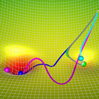
The behavior of these algorithms can be visualized below. AdaGrad (white) and RMSProp (green) are both faster and more stable than Momentum (as it chooses a better path), but they get stuck in a local minimum (since they solve Problem 2 and not Problem 1).

Momentum (magenta) with m = 0.99 vs. Gradient Descent (cyan) vs. AdaGrad (white) vs RMSProp (green) with decay rate = 0.9 on a surface with a global minimum (the left well) and local minimum (the right well)

Adam

Adaptive Moment Estimation (Adam) combines RMSProp and Momentum (getting the best of two worlds!). In AdaGrad and RMSProp, with a decay rate closer to one, the sum of squared gradients would be very small in the initial iterations (the moments are biased towards zero), leading to a very high learning rate at the beginning. We overcome this problem using bias correction.

# Adam
m1 = 0
m2 = 0
for t in range(num_steps):
   m1 = (beta1 * m1) + (1 - beta1) * dw
   m2 = (beta2 * m1) + (1 - beta2) * dw * dw
   m1_unbias = m1 / (1 - beta1 ** t)
   m2_unbias = m2 / (1 - beta2 **t)
   w += -learning_rate * m1_unbias / (m2_unbias.sqrt() + 1e-7)

Beta1 is the decay rate for the first moment, the sum of gradient (aka momentum), commonly set at 0.9. Beta 2 is the decay rate for the second moment, the sum of gradient squared, and it is commonly set at 0.999.

Adam has become a go-to optimizer for most of the deep learning community today. Learning rates = 1e-3, 5e-4, and 1e-4 can be a great starting point for most models.

Momentum (magenta) with m = 0.99 vs. Gradient Descent (cyan) vs. AdaGrad (white) vs RMSProp (green) with decay rate = 0.9 vs Adam (blue) with beta1 = 0.9 and beta2 = 0.999 on a surface with a global minimum (the left well) and local minimum (the right well)

Credits: I have created these visualizations using this visualization tool.
You can also look at this cool visualization I came across on Emilien Dupont's blog post, where you can click anywhere on the loss profile to see how different methods converge from that starting point.