Generative Modeling with Variational Autoencoders
Till now, I have talked about supervised learning where our model is trained to learn a mapping function of data $\mathbf{x}$ to predict labels $\mathbf{y}$, for example, the tasks of classification, object detection, segmentation, image captioning, etc. However, supervised learning requires large datasets that are created with human annotations to train the models.
The other side of machine learning is called unsupervised learning where we just have data $\mathbf{x}$, and the goal is to learn some hidden underlying structure of the data using a model. Through this approach, we aim to learn the distribution of the data $p(\mathbf{x})$ and then sample from it to generate new data, in our case images.
Autoencoders
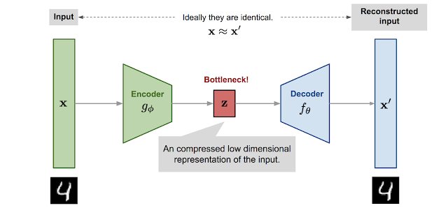
An autoencoder is a bottleneck structure that extracts features $\mathbf{z}$ from the input images $\mathbf{x}$ and uses them to reconstruct the original data $\mathbf{x}'$, learning an identity mapping.
- Encoder: network that compresses the input into a latent-space representation (of a lower dimension)
- Decoder: network that reconstructs the output from this representation
Since we want the autoencoder to learn to reconstruct the input data, the loss objective is a simple L2-loss between the input and the reconstructed output $\mathbf{x}' = f_\theta(g_\phi(\mathbf{x}))$. \begin{equation*} L_\text{AE}(\theta, \phi) = || \mathbf{x} - f_\theta(g_\phi(\mathbf{x})) ||_2^2 \tag{1} \end{equation*}
This approach is used for learning a lower-dimensional feature representation from the training data that captures meaningful factors of variation in it. After training, we get rid of the decoder and use the encoder to obtain features that contain useful information about the input that can be used for downstream tasks.
Autoencoders are generally used for dimensionality reduction (or data compression) and to initialize a supervised model. Since it is not probabilistic, we cannot sample new data from the learned model, and new images cannot be generated$^*$.
Variantional Autoencoders (VAEs)
VAEs, introduced in Auto-Encoding Variational Bayes paper are a probabilistic version of autoencoder that lets you sample from the model to generate new data. Instead of mapping the input into a fixed vector, we want to map it into a distribution, denoted as $p_\theta$.
- Prior $p_\theta (\mathbf{z})$: Prob distribution over the latent variables (fixed and often assumed to be a simple Gaussian)
- Posterior $p_\theta (\mathbf{x}|\mathbf{z})$: Prob distribution over images conditioned on the latent variables
- Likelihood $p_\theta (\mathbf{z}|\mathbf{x})$: Prob distribution over latent variables given input data
Assuming that we know the real parameter $\theta^*$ for this distribution, we can generate new samples for a real data point $\mathbf{x}^{(i)}$ as,
- First, sample a $\mathbf{z}^{(i)}$ from a true prior distribution $p_{\theta^*}(\mathbf{z})$.
- Feed it into the decoder model to obtain the posterior $p_{\theta^*}(\mathbf{x} \vert \mathbf{z} = \mathbf{z}^{(i)})$.
- Then sample a new data point $\mathbf{x'}^{(i)}$ from this true posterior.
As you would be wondering a neural network cannot output a probability distribution so, instead the decoder predicts the mean $\mu_{\mathbf{x} \vert \mathbf{z}}$ and diagonal variance $\Sigma_{\mathbf{x} \vert \mathbf{z}}$ of the posterior, assuming it to be also Gaussian such that $p_\theta (\mathbf{x}|\mathbf{z}) = \mathcal{N}(\mu_{\mathbf{x} \vert \mathbf{z}}, \Sigma_{\mathbf{x} \vert \mathbf{z}})$.
There is an inherent assumption here that the pixels of the generated image are conditionally independent given the latent variable and this is the reason why VAEs tend to generate blurry images.
In order to estimate the true parameter $\theta^*$, we learn the model parameters that maximize the probability of generating real data samples (maximum likelihood estimation), \begin{align*} \theta^{*} &= \arg\max_\theta \prod_{i=1}^n p_\theta(\mathbf{x}^{(i)}) \\ &= \arg\max_\theta \sum_{i=1}^n \log p_\theta(\mathbf{x}^{(i)}) \tag{2} \end{align*}
Before moving further, let's see how we can obtain the distribution of the data $p_\theta(\mathbf{x})$.
-
Marginalize out the latent variable to simplify as, \begin{align*} p_\theta(\mathbf{x}) &= \int p_\theta(\mathbf{x}, \mathbf{z}) d\mathbf{z} = \int \underbrace{p_\theta(\mathbf{x}\vert\mathbf{z})}_{\text{posterior}} \; \underbrace{p_\theta(\mathbf{z})}_{\text{prior}} d\mathbf{z} \\ \end{align*}
The terms in the integral - prior (fixed) and posterior (estimated by the decoder) are straightforward to compute. However, it is impossible to integrate over all $\mathbf{z}$ as it is expensive to check all the possible values of $\mathbf{z}$ and sum them up.
-
Another idea is to use Baye's rule, \begin{align*} p_\theta(\mathbf{x}) = \frac{p_\theta(\mathbf{x}\vert\mathbf{z}) \; p_\theta(\mathbf{z})}{p_\theta(\mathbf{z}\vert\mathbf{x})} \approx \frac{p_\theta(\mathbf{x}\vert\mathbf{z}) \; p_\theta(\mathbf{z})}{q_\phi(\mathbf{z}\vert\mathbf{x})} \end{align*}
The numerator has the same terms as above. The denominator has the likelihood term that can be approximated by another neural network (encoder) as $q_\phi(\mathbf{z}\vert\mathbf{x}) \approx p_\theta (\mathbf{z}|\mathbf{x})$.
Again, we assume that is follows a Gaussian distribution as $q_\phi (\mathbf{z}\vert\mathbf{x}) = \mathcal{N}(\mu_{\mathbf{z} \vert \mathbf{x}}, \Sigma_{\mathbf{z} \vert \mathbf{x}})$, and the encoder predicts the mean $\mu_{\mathbf{z} \vert \mathbf{x}}$ and diagonal variance $\Sigma_{\mathbf{z} \vert \mathbf{x}}$.
The encoder, therefore, outputs a distribution of latent variables $\mathbf{z}$ given the input data $\mathbf{x}$. The training process looks like,
- Input a real data point $\mathbf{x}^{(i)}$ to the encoder to obtain the likelihood $q_\phi (\mathbf{z}\vert\mathbf{x} = \mathbf{x}^{(i)})$.
- Sample a latent variable from this likelihood $\mathbf{z}^{(i)} \sim \mathcal{N}(\mu_{\mathbf{z} \vert \mathbf{x}}, \Sigma_{\mathbf{z} \vert \mathbf{x}})$
- Feed it into the decoder to obtain the posterior $p_{\theta^*}(\mathbf{x} \vert \mathbf{z} = \mathbf{z}^{(i)})$.
- Then sample a new data point from this posterior $\mathbf{x'}^{(i)} \sim \mathcal{N}(\mu_{\mathbf{x} \vert \mathbf{z}}, \Sigma_{\mathbf{x} \vert \mathbf{z}})$
Sampling is a stochastic process and therefore we cannot backpropagate the gradient. To make it trainable, the reparameterization trick is introduced such that, \begin{align*} \mathbf{z} &\sim q_\phi(\mathbf{z}\vert\mathbf{x}^{(i)}) = \mathcal{N}(\mathbf{z}; \boldsymbol{\mu}^{(i)}, \boldsymbol{\sigma}^{2(i)}\boldsymbol{I})\\ \mathbf{z} &= \boldsymbol{\mu} + \boldsymbol{\sigma} \odot \boldsymbol{\epsilon} \text{, where } \boldsymbol{\epsilon} \sim \mathcal{N}(0, \boldsymbol{I}) \end{align*} where $\odot$ refers to an element-wise product.
Deriving ELBO Loss
In order to obtain the loss objective of a VAE, we further simpify Equation 2 by first multipying $1 = \int q_\phi(\mathbf{z}\vert\mathbf{x}^{(i)}) \; dz$ with $\log p_\theta(\mathbf{x}^{(i)})$ and then solving, \begin{align*} \log p_\theta(\mathbf{x}^{(i)}) &= \log p_\theta(\mathbf{x}^{(i)}) \int q_\phi(\mathbf{z}\vert\mathbf{x}^{(i)}) \; dz = \int q_\phi(\mathbf{z}\vert\mathbf{x}^{(i)}) \log p_\theta(\mathbf{x}^{(i)}) \; dz \\ &=\mathbf{E}_{\mathbf{z}\sim q_\phi(\mathbf{z}\vert\mathbf{x}^{(i)})} [\log p_\theta(\mathbf{x}^{(i)})] \\ \\ &\text{applying Baye's rule,}\\ &= \mathbf{E}_{\mathbf{z}\sim q_\phi(\mathbf{z}\vert\mathbf{x}^{(i)})} \left[ \log \frac{p_\theta(\mathbf{x}^{(i)}\vert\mathbf{z}) \; p_\theta(\mathbf{z})}{p_\theta(\mathbf{z}\vert\mathbf{x}^{(i)})} \right] \\ \\ &\text{multipy & divide by same term}\\ &= \mathbf{E}_{\mathbf{z}\sim q_\phi(\mathbf{z}\vert\mathbf{x}^{(i)})} \left[ \log \frac{p_\theta(\mathbf{x}^{(i)}\vert\mathbf{z}) \; p_\theta(\mathbf{z})}{p_\theta(\mathbf{z}\vert\mathbf{x}^{(i)})} \frac{q_\phi(\mathbf{z}\vert\mathbf{x}^{(i)})}{q_\phi(\mathbf{z}\vert\mathbf{x}^{(i)})} \right] \\ \\ &\text{rearranging}\\ &= \mathbf{E}_{\mathbf{z}\sim q_\phi(\mathbf{z}\vert\mathbf{x}^{(i)})} \left[ \log p_\theta(\mathbf{x}^{(i)}\vert\mathbf{z}) \right] + \mathbf{E}_{\mathbf{z}\sim q_\phi(\mathbf{z}\vert\mathbf{x}^{(i)})} \left[ \frac{p_\theta(\mathbf{z})}{q_\phi(\mathbf{z}\vert\mathbf{x}^{(i)})} \right] + \mathbf{E}_{\mathbf{z}\sim q_\phi(\mathbf{z}\vert\mathbf{x}^{(i)})} \left[ \frac{q_\phi(\mathbf{z}\vert\mathbf{x}^{(i)})}{p_\theta(\mathbf{z}\vert\mathbf{x}^{(i)})} \right] \\ &= \mathbf{E}_{\mathbf{z}\sim q_\phi(\mathbf{z}\vert\mathbf{x}^{(i)})} \left[ \log p_\theta(\mathbf{x}^{(i)}\vert\mathbf{z}) \right] - \mathbf{D}_{KL}\left( q_\phi(\mathbf{z}\vert\mathbf{x}^{(i)}) \; || \; p_\theta(\mathbf{z}) \right) + \underbrace{\mathbf{D}_{KL} \left( q_\phi(\mathbf{z}\vert\mathbf{x}^{(i)}) \; || \; p_\theta(\mathbf{z}\vert\mathbf{x}^{(i)}) \right)}_{\text{cannot be computed but KL-Divergence} \ge 0 \text{ always}} \\ &\ge \underbrace{\mathbf{E}_{\mathbf{z}\sim q_\phi(\mathbf{z}\vert\mathbf{x}^{(i)})} \left[ \log p_\theta(\mathbf{x}^{(i)}\vert\mathbf{z}) \right]}_{\text{reconstruction term}} - \underbrace{\mathbf{D}_{KL} \left( q_\phi(\mathbf{z}\vert\mathbf{x}^{(i)}) \; || \; p_\theta(\mathbf{z}) \right)}_{\text{prior matching term}} \end{align*}
The first term is the data reconstruction term that measures the reconstruction likelihood of the decoder from our variational distribution. It ensures that the learned distribution is modeling effective latents that the original data can be regenerated from.
The second term measures how similar the learned variational distribution is to a prior belief held over latent variables. Since both the distributions are Gaussians, KL-divergence can be computer in closed form.
This gives us a lower bound on the log-likelihood of the data and we jointly train both the encoder and decoder to maximize it. \begin{align*} \theta^{*} &= \arg\max_\theta \sum_{i=1}^n \log p_\theta(\mathbf{x}^{(i)}) \\ &\ge \arg\max_{\theta, \phi} \sum_{i=1}^n \mathbf{E}_{\mathbf{z}\sim q_\phi(\mathbf{z}\vert\mathbf{x}^{(i)})} \left[ \log p_\theta(\mathbf{x}^{(i)}\vert\mathbf{z}) \right]- \mathbf{D}_{KL}(q_\phi(\mathbf{z}\vert\mathbf{x}^{(i)}) \; || \; p_\theta(\mathbf{z})) \end{align*} It is known as the variational lower bound, or evidence lower bound (ELBO).
The loss function (that we minimize) is given as, \begin{equation*} L_{\text{VAE}}(\theta, \phi) = - \mathbf{E}_{\mathbf{z}\sim q_\phi(\mathbf{z}\vert\mathbf{x})} \left[ \log p_\theta(\mathbf{x}\vert\mathbf{z}) \right] + \mathbf{D}_{KL}\left( q_\phi(\mathbf{z}\vert\mathbf{x}) \; || \; p_\theta(\mathbf{z}) \right) \tag{3} \end{equation*}
$*$ - I have tried generating new images using an autoencoder by first obtaining the latent representation of two images and then performing the reconstruction on the linear interpolation between them. Below are the results on the CIFAR10 dataset, with the first two columns showing original images and the last one showing the new image.


Comments
Post a Comment