ResNet: The Revolution of Depth

In 2015, Batch Normalization was discovered, which heralded the progress of architectures as it was now possible to train deep networks without using any tricks - allowing us to use much higher learning rates and be less careful about initialization. It also acts as a regularizer, eliminating the need for Dropout.

Another major problem with deep networks was of vanishing/exploding gradients, but it was now being handled by Kaiming Initialization. With the stage set in place, experiments began on training deeper models.

It was noted that when deeper networks are able to start converging, a degradation problem occurs: as we increase the depth, the accuracy gets saturated (which might be unsurprising) and then degrades rapidly. Unexpectedly, such degradation is not caused by overfitting (which was the initial guess), because adding more layers to a suitably deep model lead to higher training error. It turns out, deeper networks are underfitting!

By intuition, it is expected that deeper models should do at least as good as shallow models, as they can emulate the shallower model by copying layers from it and setting the other extra layers to identity. Since the deeper models are underfitting, it shows that there is a problem in optimization and somehow these deeper networks are not able to learn the identity functions.

A solution to this is to change the design of the network so that it is easy for it to learn the identity functions on unused layers. This forms the idea of a residual block shown below.

In order to learn the identity function, the weights of the two convolutions are set to zero. It is easier to push the residual to zero during learning than to fit an identity mapping.

These connections are often called skip connections and they neither add extra parameters nor computational complexity. Residual blocks can still be trained end-to-end by SGD with backpropagation (there is no need for any kind of modification). A residual network (or ResNet) is formed by stacking many such residual blocks.

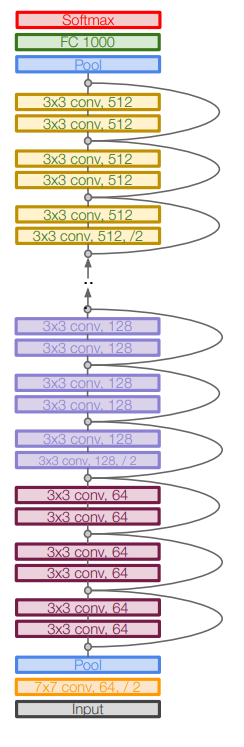
Architecture: Similar to VGG, ResNet is divided into 4 stages with a different number of residual blocks. The design principles are fixed as,

• Each residual block has two $3 \times 3$ convolution layers.
• After each stage, the number of channels is doubled (starting with 64 and going to 512)
• After each stage, the spatial dimension is reduced by half using a stride of 2 in the first conv of the next stage.

Whenever the channel dimension is increased, the spatial dimension is decreased proportionally (was done with a max-pool layer in VGG), so as to preserve the time complexity per layer.

When the stage changes, the dimension of the input to skip connection becomes different from the output. In such a case, a $1 \times 1$ conv (with a stride of 2) is added to the input to match the dimensions. The output then becomes: \begin{equation*} \text{H(x) = F(x) + W x} \end{equation*} where $W$ is a learnable parameter called projection shortcut. These are used only for changing dimensions, other shortcuts are identity.

Each convolution is followed by a BatchNorm layer and a ReLU non-activation.

Like GoogleNet, ResNet uses an aggressive stem network to downsample the image input 4x before applying the residual blocks. It also does not have fully-connected layers, instead uses global average pooling followed by a single linear layer (with softmax) to generate class scores.

The authors presented two variants, ResNet-18 and ResNet-34.

As the 34-layer network performed better than the 18-layer one, it was clear that adding even more layers would mean better performance. However, adding more layers would also bring more computation costs.

Taking inspiration from GoogleNet, the authors added bottleneck layers in each residual block. The bottleneck block accepts 4 times the channel dimension as a basic block and works with lower computation costs even with an extra added layer per block.

Replacing all the basic blocks in ResNet-34 with bottleneck blocks would give the ResNet-50 architecture. ResNet-50 is an excellent baseline architecture for many tasks today! Similarly using a different number of bottleneck blocks in different stages, the authors present ResNet-101 and ResNet-152 variants.

Training: The model was trained on the Cross-entropy loss function using stochastic gradient descent with a batch size of 256 examples, a momentum of 0.9, and a weight decay of 0.0001. The learning rate starts from 0.1 and is divided by 10 when the error plateaus.

The weights were initialized using Kaiming initialization. No dropout was used.

ResNet was the first architecture to have crossed the human error rate and won 1st place on ImageNet detection, ImageNet localization, COCO detection, and COCO segmentation in 2015.

Important design choices of the paper are,

• 4 Stages, Bottleneck residual blocks (conv layers with skip connections)
• Number of channels stage-wise: 64, 128, 256, 512
• Batch Normalization used
• Activation Function: ReLU
• Data pre-processing: subtract per-pixel mean
• Weight Initialization: Kaiming
• Regularization: L2 Weight decay ($\lambda$ = 1e-4)
• Learning rate: 0.1 and reduced (divided by 10) when error plateaus
• Optimization Method: SGD + Momentum (m=0.9) with batch size of 256
• Loss function: Cross-Entropy loss

Link to the paper: Deep Residual Learning for Image Recognition