Probabilistic Movement Primitives Part 3: Supervised Learning

In this post, we describe how a Probabilistic Movement Primitive can be learnt from demonstrations using supervised learning.

Learning from Demonstrations

To simplify the learning of the parameters $\theta$, a Gaussian is assumed for $p(w; \theta) = \mathcal{N}(w | \mu_w, \Sigma_w)$ over $w$. The distribution $p(y_t| \theta)$ for time step $t$ is written as,

\begin{equation} \begin{aligned} p(y_t| \theta) & = \int p(y_t| w) \; p(w; \theta) dw, \\ & = \int \mathcal{N}(y_t | \Phi_t w, \Sigma_y) \; \mathcal{N}(w | \mu_w, \Sigma_w), \\ & = \mathcal{N}(y_t | \Phi_t \mu_w, \Psi_t \Sigma_w \Phi_t^T + \Sigma_y). \end{aligned} \end{equation}

It can be observed from the above equation, that the learnt ProMP distribution is Gaussian with, \begin{equation} \mu_t = \Phi_t \mu_w, \hspace{10mm} \Sigma_t = \Phi_t \Sigma_w \Phi_t^T + \Sigma_y \end{equation}

Learning Stroke-based Movements

For stroke-based movements, the parameter $\theta = \{ \mu_w, \Sigma_w \}$ which specifies the mean and variance of $w$, can be learnt by maximum likelihood estimation using multiple demonstrations. The weights of each trajectory are estimated individually with linear ridge regression,

\begin{equation} w_i = (\Phi^T \Phi + \lambda I)^{-1} \Phi^T Y_i \end{equation}

where $Y_d$ represents the positions of all joints from the demonstration $d$ for all time steps, $\Phi$ represents the basis function matrix and $I$ is the identity matrix. The demonstrations are aligned by varying the phase variable. For each demonstration, it assumed that $z_{begin}$ = 0 and $z_{end}$ = 1. The ridge factor $\lambda$ is generally set to a very small value ($\lambda = 10^{-12}$), as larger value debases the estimation of the trajectory distribution.

The mean $\mu_w$ and covariance $\Sigma_w$ are computed from $w_i$ as,

\begin{equation} \mu_w = \frac{1}{N} \sum_{i=1}^N w_i, \hspace{10mm} {\Sigma}_w = \frac{1}{N-1} \sum_{i=1}^N (i_d - \mu_w)(i_d - \mu_w)^T \end{equation}

where $N$ is the number of demonstrations. Since one trajectory is generated from one demonstration, $N$ also denoted number of trajectories.

Let's code

W = []  # list that stores all the weights
mean_W  = None
sigma_W = None

mid_term = np.dot(Phi, Phi.T) + np.dot(Phi_dot, Phi_dot.T)

for demo_traj in pos_list:
    interpolate = interp1d(z, demo_traj, kind='cubic')
    stretched_demo = interpolate(z)[None,:] # strech the trajectory to fit 0 to 1

    w_d = np.dot(np.linalg.inv(mid_term + 1e-12*np.eye(n_bfs)),
    np.dot(Phi, stretched_demo.T)).T  # weights for each trajectory
    W.append(w_d.copy()) # append the weights to the list

W =  np.asarray(W).squeeze()

mean_W = np.mean(W, axis=0)
sigma_W = np.cov(W.T)

# Computing the mean and sigma of the sampled trajectory
mean_of_sample_traj = np.dot(Phi.T, mean_W)
sigma_of_sample_traj = np.dot(np.dot(Phi.T, sigma_W), Phi) + 1e-10  # Sigma_y

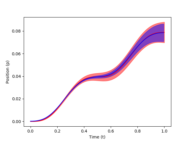
The learnt stroke-based ProMP distribution is shown in blue over the demonstration distribution in red.

References: 

1. Paraschos, Alexandros, et al. "Using probabilistic movement primitives in robotics." Autonomous Robots 42.3 (2018): 529-551.