Dynamic Movement Primitives (DMPs)
Robot manipulation and motion planning often take place in continuous state-action space where the objective is to define a desired trajectory that reaches a particular goal state. Movement Primitives (MPs) is a well established approach that formalizes the the learning of coordinated movements from Learning from Demonstrations (LfD). One primitive creates a family of movements that all converge to the same goal called a attactor point, which solves the problem of generalization.
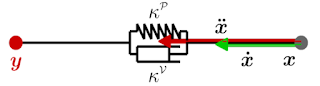
Dynamic Movement Primitives (DMPs) are learnable non-linear attractor systems that can produce both discrete as well as repeating trajectories. The theory behind DMPs is well described in this post. Consider a spring damper system shown below.

General motion equation of this system can be written as: $\ddot{x} = K^p [y - x] - K^v \dot{x}$, where $K^p$ is the spring constant and $K^V$ damps the system. A spring-damper system is used because of its ability to converge to the goal state after excitation in a finite amount of time as shown in the step response above. Therefore, the movement would always converge to the goal location irrespective of the starting position, making it a one-point attractor system. This equation is presented in a slightly different form (x is interchanged with variable y) in studies as,
\begin{equation} \tau \ddot{y} = \alpha_z ( \beta_z (g - y) ) - \dot{y}), \label{eq1} \end{equation}
where $\tau$ is the duration of movement or time constant, $g$ is the goal state and $y, \dot{y}, \ddot{y}$ are the desired position, velocity and acceleration respectively. $\alpha_z$ and $\beta_z$ are constants that replace $K^P$ and $K^V$, which keeps the system critically damped so that $y$ can monotonically converge to $g$. This equation represents a second-order linear system with unique point attractor at $(z,y) = (0, g)$ which is globally stable. Since most of the motor control problems are described by a second-order differential equation, it makes sense to use this system. However, this equation is still trivial as it would result in trajectories of similar shapes. For generating more complex movements, we add a non-linear perturbation in this system.
\begin{equation} \begin{aligned} \tau \ddot{y} = \alpha_z ( \beta_z (g - y) ) - \dot{y}) + f, \end{aligned} \label{eq3} \end{equation}
This equation is called the transformation system since it transforms a simple linear system into a desired nonlinear behavior using the nonlinear forcing function $f$. A DMP is therefore a stable dynamical system that enables reproduction of complex trajectories through a spring-damper system modulated with a nonlinear function. The forcing function $f$ is defined as a linear combination of the basis function as,
\begin{equation} f(t) = \frac{\sum_{i=1}^{N} \Psi_i(t) w_i}{\sum_{i=1}^{N} \Psi_i(t)}, \label{eq4} \end{equation}
where $\Psi$ denotes a basis function and $\omega$ denotes represents the adjustable weight. Tweaking this forcing function $f$ gives rise to varied trajectories and is responsible for generating stroke (point-to-point) or rhythmic (repeating) movements. The former is generated by choosing $f$ to be phasic (similar to a point attractor), whereas the latter is generated by choosing $f$ to be periodic. Basis functions enable smooth reproduction of movements and are defined beforehand by trial and error. On the other hand, the weights have to learnt by supervised learning as these parameters are linear.
Discrete movements
For deriving discrete movements (i.e. point attractor), a phase variable $x$ is introduced as a replacement of time $t$.
\begin{equation} \begin{aligned} & \tau \dot{x}(t) = - \alpha_x x(t), \\ \text{Solution: } & x = x_0 \text{ exp} (-\alpha_x \frac{t}{\tau}).). \end{aligned} \label{eq5} \end{equation}
where $\alpha_x$ is a constant fine-tuned such that the system is stable. This equation is called the canonical system as it models the generic behavior of our model equations. Its solution shows that the system will exponentially converge to zero as the time reaches infinity irrespective of the positive initial value $x_0$. We write the forcing function for discrete movements as,
\begin{equation} \begin{aligned} & f(x) = \frac{\sum_{i=1}^{N} \Psi_i(x) w_i}{\sum_{i=1}^{N} \Psi_i(x)} x (g - y_0), \\ & \Psi_i(x) = \text{exp}(-\frac{1}{2 \sigma_i^2}(x - c_i)^2). \end{aligned} \label{eq6} \end{equation}
where $y_0$ is the initial state and $g$ is the goal state. The $N$ exponential basis functions $ \Psi_i(x)$ are defined as Gaussian kernels where $\sigma_i$ and $c_i$ defines the width and the centre of the basis function. It should be noted that this system converges to the globally stable point-attractor $(x,y,z) = (0,g,0)$ as the time reaches infinity. Further, the forcing term goes to zero at $g = y_0$, as it becomes unnecessary once the goal is reached.
Rhythmic movements
For generating rhythmic movements (i.e. limit cycle) , the periodicity can be introduced in either the basis functions or the canonical system. Here, we present the latter approach of using canonical system as a simple harmonic oscillator.
\begin{equation} \tau \dot{\phi} = 1, \label{eq7} \end{equation}
where $\phi \in [0, 2\pi]$ is the phase angle of the oscillation in polar coordinates. The forcing function for rhythmic movement is represented as,
\begin{equation} \begin{aligned} & f(\phi, r) = \frac{\sum_{i=1}^{N} \Psi_i(\phi) w_i}{\sum_{i=1}^{N} \Psi_i(\phi)} r, \\ & \Psi_i(\phi) = \text{exp}(-h_i(cos(\phi - c_i) - 1). \end{aligned} \label{eq8} \end{equation}
where $r$ is the amplitude of oscillation. The basis functions are represented as von-Mises basis for generating rhythmic movements, which are very similar to Gaussian functions but are periodic.
References:


Comments
Post a Comment