Probabilistic Movement Primitives Part 2: Phase variable and Basis functions

As a continuation of our series on ProMPs, we will introduce the concepts of phase variable and basis functions in this post.

Temporal Modulation

The execution speed of the movement can be adjusted with temporal modulation. A phase variable $z$ is introduced (similar to the DMP approach) to separate the movement from the time signal. We can vary the speed of the movement by regulating the rate of phase variable. The phase is defined as $z_0 = 0$ at the start of the movement and $z_T = 1$ at the end (so as to normalize it). Phase defines how quickly the time evolves for a trajectory. The basis function $\phi(t)$ now directly depend on the phase instead of time, \begin{equation} \phi_t = \phi(z_t), \; \; \; \dot{\phi}_t = \dot{\phi}(z_t) \dot{z}_t. \label{eq12} \end{equation}

Let's code

We choose a monotonically increasing function with time that starts at 0 and ends at 1. By default, the phase speed is taken as 1.

def get_phase_variables(phase_speed):
    phase_start = 0
    time_steps = int(num_points/phase_speed) 
    phase_end = 1

    Dz = np.ones(time_steps)*phase_speed  # derivative of phase variable z dot
    phase_z  = np.cumsum(Dz)*dt  # phase variable z
    return phase_z, Dz

def get_phase_from_time(time_step):
    phase_end = 1
    return time_step/phase_end

Rhythmic and Stroke-Based Movements

Similar to DMPs, we choose the basis functions depending upon the type of movement. Gaussian basis functions $b_i^G$ is used for generating stroke-based movements, while Von-Mises basis functions $b_i^{VM}$ is used to generate rhythmic movements such that, \begin{equation} b_i^G(z) = \text{exp } \left( -\frac{(z_t - c_i)^2}{2h} \right), \end{equation} \begin{equation} b_i^{VM}(z) = \text{exp } \left( \frac{\text{cos}(2\pi (z_t - c_i))}{h} \right), \end{equation} where $h$ represents the width and $c_i$ represents the center for the $i$th basis function. These basis functions are normalized to improve the regression's performance as, \begin{equation} \phi_i(z_t) = \frac{b_i(z)}{\sum_{j=1}^K b_j(z)}. \label{eq15} \end{equation}

Let's code

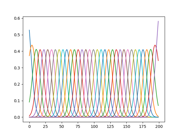
For our case of learning a stroke-based ProMP, 35 radial basis function are defined with variance of $0.0286$ . The centres of this basis functions are placed evenly spaced between 0 and 1. With a default phase speed of 1, taking each time step at 0.005 results in 200 time steps for the full trajectory.

  
n_bfs = 35 # number of basis function
bfs_sigma = 0.0286 # variance of the basis function
bfs_centres = np.linspace(0, 1, n_bfs) # centers of the basis function

def generate_basis_function(phase_z, phase_zd):
    phase_minus_centre = np.array(map(lambda x: x - bfs_centres,
    np.tile(phase_z, (n_bfs, 1)).T)).T

    Phi   = np.exp(-0.5 *np.power(phase_minus_centre/bfs_sigma, 2))
    PhiD  = np.multiply(Phi,  -phase_minus_centre/(bfs_sigma)) * phase_zd 

    # normalization
    sum_bfs    = np.sum(Phi,   axis=0)
    sum_bfsD   = np.sum(PhiD,  axis=0)
    
    PhiD_normalized = ( (PhiD * sum_bfs - Phi * sum_bfsD) * 1./np.power(sum_bfs, 2) ) 
    Phi_normalized  = Phi/sum_bfs[None, :]
    return Phi_normalized, PhiD_normalized
    
# Generate the Basis Function for the default phase speed = 1
z, z_dot = get_phase_variables(1)
Phi, Phi_dot = generate_basis_function(z, z_dot)

The radial basis functions generated from the above code are shown in the Figure below.

References: 

1. Paraschos, Alexandros, et al. "Using probabilistic movement primitives in robotics." Autonomous Robots 42.3 (2018): 529-551.