Markov Decision Processes Part 2: Discounting
As discussed in the previous post, four main components of a MDP include state, action, model and rewards. In MDPs, rather than focusing on immediate rewards, the agent tries to maximize the total future reward. A particular action might yield higher immediate reward, but it might not be best in the long term. This makes it challenging to find an optimal policy for a MDP. To proceed in this direction, we need to calculate the expected cumulative reward an agent would receive in the long run and then choose an action with the maximum expected value.
In this post, we will formulate a way to calculate the cumulative reward an agent would receive in the long term, denoted by Gt. It is also called a return. If the sequence of rewards earned after time step t is denoted by Rt+1, Rt+2, Rt+3, and so on, then the return is given by
Gt = Rt+1 + Rt+2 + Rt+3 + ..... + RT
Where T is the final time step. If a MDP does not have an end-state or a terminal state, then, the return is equal to
Gt = Rt+1 + Rt+2 + Rt+3 + ..... + inf
This is very straightforward and hence self-explanatory. But the formula defined above has some shortcomings. Let me explain it to you with the help of a real-world scenario. You have to select one of the two given options :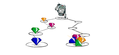
Option 1 - I will give you one chocolate every day for ten days.
Option 2 - I promise you to give ten chocolates after ten days.
Which option will you choose? You will obviously choose option 1, primarily because of the presence of uncertainty in option 2. You tend to prefer things right away rather than waiting for it because you never know what might happen later (What if I go bankrupt and cannot buy you the ten chocolates I promised).
In the picture below, an agent is provided with two different paths to choose from. In the left path, the robot gets the diamonds in each step and in the other one, it gets all the diamonds at the end. If we apply the equation described above, we will get the same returns in both cases. But, the above discussion tells us that this should not be the case. We prefer to accrue earlier rewards more than later rewards. Sooner rewards have a higher utility than later rewards.
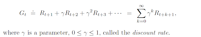
In order to formalize this, we use the concept of discounting. Discounting makes sure that our agents would prefer getting rewards earlier rather than later. In this concept, we decay the value of later rewards exponentially so that they worth lesser than the earlier rewards. Discounting factor is denoted by γ (gamma) = [0,1]. The discount rate determines the present value of future rewards. The future rewards are discounted because of the presence of uncertainty. Farther away the reward is in the future, more the uncertainty and hence more is it's discounting. The modified equation for the return is given by,
For a value of γ = 0, the agent is short-sighted, i.e. it is only concerned with immediate reward. All future rewards are neglected in this case. For a value of γ very close to 1, the agent becomes more far-sighted and takes into consideration all rewards almost equally. For a continuous task where there is no terminal state, the use of discounting is very useful. For a value of γ between 0 and 1, Gt forms a geometric progression whose sum is finite.
References:
1. CS188 Introduction to Artificial Intelligence, UCB
2. Sutton, R. S., & Barto, A. G. (2018). Reinforcement learning: An introduction. MIT press.


Comments
Post a Comment