YA's Blog

Legged robots are an attractive option to wheeled robots primarily for applications in rough terrain and difficult, cluttered environments. The freedom to choose contact points enables such robots to interact with the environment while avoiding obstacles effectively. With such capabilities, legged robots may be applied to application such as rescuing people in mountains and forests, climbing stairs, carrying payloads in construction sites, and inspecting unstructured under-ground tunnels. Designing dynamic and agile locomotion for such robots is a longstanding research problem because it is difficult to control an under-actuated robot performing highly dynamic motion that requires tricky balance. The recent advances in Deep Reinforcement Learning (DRL) has made it possible to learn robot locomotion policies from scratch without any human intervention. In this post, we discuss various research directions where DRL can be employed to solve locomotion problems in quadruped robots. Si

Reinforcement learning has gained popularity after the success of agents playing Atari games at superhuman level. Applying RL for solving intelligent decision making problems in robotics is a key to building smarter robots. In this post, we briefly discuss how an MDP can be defined for a robot and talk about Deep Reinforcement learning and its shortcomings. Markov Decision Process(MDP) Reinforcement learning agents learn actions from scratch through their interactions with the environment. There are four basic components of a reinforcement learning system: states, actions, reward and policy. The state in RL is defined by the current configuration or the state of the robot. For example, the current sensor readings such as motor encoder values or position and orientation of the centre of mass of the robot can be taken to define the "state space". The actions comprises of the possible motions of the robot in response to its interaction with the environment. The action space

Since two posts we have been talking about MDPs. As discussed in the previous post, the ultimate goal of a MDP is to maximize the total future reward. In the last post, we had calculated the cumulative sum of the long-term rewards (G t ). In this post, we will calculate the expected long-term reward which the agent has to maximize.  A value of a state is the total amount of reward an agent can expect to accumulate over the future, starting from that state. A value function computes the value of a state. A value of state gives us an estimate of how good the state is to be in. The value of a state should not be confused with rewards. A reward signal indicates what is good in an immediate sense, whereas a value function specifies what is good in the long run. For example, a state might always yield a low immediate reward but still have a high value because it is regularly followed by other states that yield high rewards. Since our goal is to maximise long-term reward, we take into account

As discussed in the previous post, four main components of a MDP include state, action, model and rewards. In MDPs, rather than focusing on immediate rewards, the agent tries to maximize the total future reward. A particular action might yield higher immediate reward, but it might not be best in the long term. This makes it challenging to find an optimal policy for a MDP. To proceed in this direction, we need to calculate the expected cumulative reward an agent would receive in the long run and then choose an action with the maximum expected value. In this post, we will formulate a way to calculate the cumulative reward an agent would receive in the long term, denoted by G t . It is also called a return. If the sequence of rewards earned after time step t is denoted by R t+1 , R t+2 , R t+3 , and so on, then the return is given by G t = R t+1 + R t+2 + R t+3 + ..... + R T Where T is the final time step. If a MDP does not have an end-state or a terminal state, then, the return

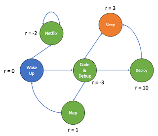
We are always solving MDPs in the back of our minds. Should I sleep right now? Should I watch Netflix? Should I code? We generally weigh our options based on returns or what is called rewards in MDPs. We always work towards gaining the highest long-term reward possible. If I watch Netflix, I loose on the hours when I could have slept or deployed by application (so negative reward). If I deploy my application, I could make more money(greater positive reward). If I sleep or take a nap, I am improving my health(a lesser positive reward). And that's exactly what a MDP is!    The word "Markov" means that the action-outcome depends only on the current state that an agent is in. It is independent of the future or past states. Therefore, the next state will only be dependent on the current state. The basic framework of a MDP is defined below : States: S Actions: A(s) Model : T(s,a,s') ~ P(s' | s,a) Reward: R(s) --------------------------------------------