Occupany Grid Mapping

In order to map out an unknown environment for future reference, a robot uses the Simultaneous Localization And Mapping (SLAM) algorithm. We talked about solving the localization problem using Filtering in the previous posts. In this post, we will look at the mapping problem. We will assume that we know the position/orientation of the robot in the 3D world (which we obtain from filtering), and want to build a map of the objects in the world.

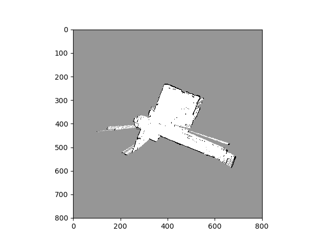
Occupancy grid map (OGM) is a very common way of representing the layout of the unknown environment. It is a large gray-scale image where each pixel represents a cell in the physical world. The cells that are occupied are colored black and empty cells represent free space are colored white. The grey cells represent unexplored areas. Before moving forward, lets make some assumptions:

• Assumption 1: each cell is either free or occupied. We model each cell as a binary random variable that indicates occupancy. Let the probability that the cell $m_i$ be occupied be $P(m_i)$, then $P(m_i) = 0$ indicates a free cell and $p(m_i) = 1$ indicates an occupied cell. A priori, we do not know the state of the cell so we will set the prior probability to be $P(m_i) = 0.5$.
  
  
• Assumption 2: the world is static. We assume that the objects in a room do not move when the mapping is carried out as we are interested in building a map of the walls inside the room.
  
  
• Assumption 3: cells are independent of each other. This means that the probability distribution of the map is given by the product of its individual cells, if cells in the map are denoted by a vector $m = (m_1, ...)$ then the map is given by, \begin{equation*} P(m) = \prod_{i} P(m_i) \end{equation*}

Estimating the map from the data

Given the robot pose $x_1, ..., x_k$ and sensor data/observations $y_1, ..., y_k$ our goal is to estimate the state of each cell $m_i \in \{0,1\}$ \begin{equation*} P(m|x_1, ..., x_k, y_1, ..., y_k) = \prod_{i} P(m_i|x_1, ..., x_k, y_1, ..., y_k) \end{equation*} We need to simplify this further to obtain a more meaningful expression using the Baye's rule $P(A|B,C) = \frac{P(B|A,C)P(A|C)}{P(B|C)}$, \begin{align*} P(m_i|y_k, y_{1:k-1}, x_{1:k}) &= \frac{P(y_k|m_i, y_{1:k-1}, x_{1:k}) P(m_i|y_{1:k-1}, x_{1:k})}{P(y_k|y_{1:k-1}, x_{1:k})} \\ &= \frac{P(y_k|m_i, x_{k}) P(m_i|y_{1:k-1}, x_{1:k-1})}{P(y_k|x_{k})} \end{align*} We use the markov property for simplification that the current observation depend only on the current state. We can further simply the term $P(y_k|m_i, x_{k})$ with same Baye's rule as, \begin{align*} P(y_k|m_i, x_{k}) = &\frac{P(m_i|y_k, x_k) P(y_k|x_k)}{P(m_i|x_k)} \\ &= \frac{P(m_i|y_k, x_k) P(y_k|x_k)}{P(m_i)} \end{align*} Since the world is static (assumption 2), the occupancy of a cell does not depend on the state $P(m_i|x_k) = P(m_i)$. Ultimately we get, \begin{equation*} P(m_i|x_{1:k}, y_{1:k}) = \frac{P(m_i|y_k, x_k) P(m_i|y_{1:k-1}, x_{1:k-1})}{P(m_i)} \tag{1} \end{equation*} This term denotes the probability that the $i^{th}$ cell is occupied.

We can obtain the odds ratio of this term- the ratio of probability that the $i^{th}$ cell is occupied to probability that the $i^{th}$ cell is not occupied (or free) as, \begin{align*} \frac{P(m_i|x_{1:k}, y_{1:k})}{P(\neg m_i|x_{1:k}, y_{1:k})} &= \frac{P(m_i|y_k, x_k)}{(1 - P(m_i|y_k, x_k))} \frac{P(m_i|y_{1:k-1}, x_{1:k-1})}{(1 - P(m_i|y_{1:k-1}, x_{1:k-1}))} \frac{1 - P(m_i)}{P(m_i)} \end{align*} Note that we could write this expression as $P(m_i)$ is a binary random variable (assumption 1), so $P(\neg m_i) = 1 - P(m_i)$. The first term incoporates the latest observation $y_k$, the second term is a recursive update (it is the same probability as the left-hand side but at the previous time step) and the third term is a prior probability of the cell being occupied/non-occupied which is equal to 1 as $P(m_i) = 0.5$ (assumption 1).

Let us rewrite this formula using the log-odds-ratio that makes implementing it particularly easy. The log-odds-ratio of the probability $p(x)$ of a binary variable $x$ is defined as, \begin{equation*} l(x) = \textrm{log}\frac{p(x)}{1 - p(x)} \end{equation*} then we can write the log-odds ratio as, \begin{align*} l(m_i|x_{1:k}, y_{1:k}) &= \underbrace{l(m_i|y_k, x_k)}_{\textrm{sensor model}} + \underbrace{l(m_i|y_{1:k-1}, x_{1:k-1})}_{\textrm{previous value}} - \underbrace{l(m_i)}_{=0} \end{align*} Therefore we update the occupancy of each cell with the value $l(m_i|y_k, x_k)$ which is called the sensor model and is different for different sensors. After recursively updating the occupany of a cell for all time steps, if $l(m_i|x_{1:k}, y_{1:k}) > 0$ for a particular cell $i$, we set the occupancy to 1 (as it means that the cell is occupied) or zero otherwise, to get the maximum-likelihood estimate of the occupancy grid.

Occupancy grids are a very popular approach to represent the environment given the poses of the robot as it travels in this environment. We can also use occupancy grids to localize the robot in a future run (which is usually the purpose of creating them).