Derivation of Particle Filter Algorithm

In this post, we look at particle filters (PFs) which are a generalization of the UKF that can handle non-Gaussian filtering distributions. When a robot uses a particle filter to localize itself, it is also called Monte Carlo localization. Just like the Unscented Transform (UT) forms the building block of the UKF, the building block of a particle filter is the idea of importance sampling.

Importance Sampling

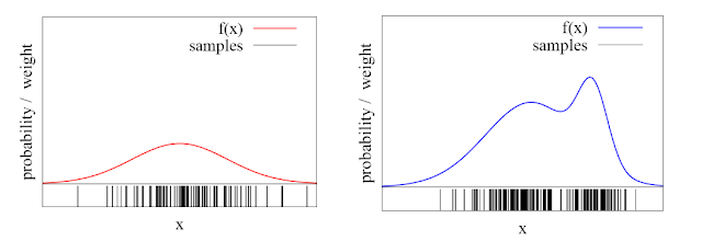
Similar to UT, the sample points have equal weights but we can approximate different probability distributions depending upon how we pick the samples $x^{(i)}$ also called “particles”, just as shown in the Figure below. The higher the number of particles in a given region, higher is the approximated probability density of that region.

Importance sampling is a technique to sample the particles to approximate a given probability distribution $p(x)$. The probability distribution is approximated as a sum of Dirac-delta distributions at points $x^{(i)}$, with weights $w^{(i)}$, \begin{equation*} p(x) \approx \sum_{i=1}^n w^{(i)} \delta_{x^{(i)}}(x) \tag{1} \end{equation*} But how do we pick these particles? The main idea is to use another known probability distribution, let us call it $q(x)$ to generate particles $x^{(i)}$ and account for the differences between the two by assigning weights to each particle, \begin{align*} &\textrm{For $i$ = 1, ..., n} \\ & x^{(i)} \sim q \hspace{5mm} \rightarrow \hspace{2mm} \textrm{Sample points from q(x)} \\ & w^{(i)} = \frac{p(x^{(i)})}{q(x^{(i)})} \tag{2} \end{align*} The original distribution $p(x)$ is called the “target” and our chosen distribution $q(x)$ is called the “proposal” (which is usually a Gaussian). If the number of particles $n$ is large, we can expect a better approximation of the target density $p(x)$.

The basic template of a PF is similar to that of the UKF and involves two steps, the first where we propagate particles using the dynamics to estimate $P(x_{k+1}|y_1, ..., y_k)$ and a second step where we incorporate the observation to compute the updated distribution $P(x_{k+1}|y_1, ..., y_{k+1})$. Consider a non-linear dynamical system with non-linear observations, \begin{align*} x_{k+1} &= f(x_k, u_k) + \epsilon \\ y_k &= g(x_k) + \upsilon \end{align*} where noise vectors $\epsilon \sim N(0,R)$ and $\upsilon \sim N(0,Q)$.

Step 1: Propagating the dynamics by one timestep

We assume that we have access to particles $x_{k|k}^{(i)}$ with equal weights $w_{k|k}^{(i)} = 1/n$, \begin{equation*} P(x_{k}|y_1, ..., y_k) \sim \frac{1}{n} \sum_{i=1}^n \delta_{x_{k|k}^{(i)}}(x) \end{equation*} Following importance sampling, we set, \begin{align*} \textrm{target : }& P(x_{k+1}|y_1, ..., y_k) \\ \textrm{proposal : } & P(x_{k}|y_1, ..., y_k) \end{align*} Then the new weights are given by (using Equation 2), \begin{align*} w_{k+1|k}^{(i)} &= \frac{P(x_{k+1}|y_1, ..., y_k)}{P(x_{k} = x_{k|k}^{(i)}|y_1, ..., y_k)} \\ &= \frac{P(x_{k+1} |x_k = x_{k|k}^{(i)},y_1, ..., y_k) P(x_k = x_{k|k}^{(i)}|y_1, ..., y_k)}{{P(x_{k} = x_{k|k}^{(i)}|y_1, ..., y_k)}} \\ &= P(x_{k+1}|x_k = x_{k|k}^{(i)}) \end{align*} This denotes the state transistion probability. The approximated target probability distrubtion can be written as (using Equation 1), \begin{align*} P(x_{k+1}|y_1, ..., y_k) &\sim \sum_{i=1}^n P(x_{k+1}|x_k = x_{k|k}^{(i)}) \delta_{x_{k|k}^{(i)}}(x) \\ &= \sum_{i=1}^n \delta_{x_{k+1|k}^{(i)}}(x) \end{align*} where the new particles are given by $x_{k+1|k}^{(i)} = f(x_{k|k}^{(i)}, u_k) + \epsilon$. Current state estimate multiplied by the transistion matrix gives us the next state estimate. Since we have a non-linear model, the particles are transformed using the non-linear dynamics function. But the term is not normalized which we fix by dividing by $n$, \begin{align*} P(x_{k+1}|y_1, ..., y_k) &\sim \frac{1}{n} \sum_{i=1}^n \delta_{x_{k+1|k}^{(i)}}(x) \\ &= \sum_{i=1}^n w_{k+1|k}^{(i)} \delta_{x_{k+1|k}^{(i)}}(x) \end{align*} We have simply rearanged the approximation such that the $1/n$ part forms the new weights and the remaining part denote the distribution of particles. Therefore this equation can be perceived as a change of location of particles whereas the weights remain unchanged.

Step 2: Incorporating the observation

Again, we follow the same procedure of importance sampling to incorporate a new observation $y_{k+1}$ by setting, \begin{align*} \textrm{target : }& P(x_{k+1}|y_1, ..., y_{k+1}) \\ \textrm{proposal : } & P(x_{k+1}|y_1, ..., y_k) \end{align*} Then the new weights are given by (using Equation 2), \begin{align*} w_{k+1|k+1}^{(i)} &= \frac{ P(x_{k+1} = x_{k+1|k}^{(i)}|y_1, ..., y_k, y_{k+1}) }{P(x_{k+1} = x_{k+1|k}^{(i)}|y_1, ..., y_k)} \\ &\propto \frac{P(y_{k+1}|x_{k+1} = x_{k+1|k}^{(i)}) P(x_{k+1} = x_{k+1|k}^{(i)}| y_1, ..., y_k)}{P(x_{k+1} = x_{k+1|k}^{(i)}|y_1, ..., y_k) } \\ &\propto P(y_{k+1}|x_{k+1} = x_{k+1|k}^{(i)}) \end{align*} This denotes the observation probability. Since we have, $y_{k+1} = g(x_{k+1}) + \upsilon$, the term $ P(y_{k+1}|x_{k+1} = x_{k+1|k}^{(i)})$ is a Gaussian such that, \begin{align*} P(y_{k+1}|x_{k+1} = x_{k+1|k}^{(i)}) &= P(\alpha_{k+1} = y_{k+1} - g(x_{k+1|k}^{(i)})) \\ &= \frac{1}{\sqrt{(2\pi)^p \textrm{det}(Q)}} \textrm{exp} \left( \frac{- \alpha_{k+1}^T Q^{-1} \alpha_{k+1}}{2} \right) \end{align*} The approximated target probability distribution can be written as (using Equation 1), \begin{align*} P(x_{k+1}|y_1, ..., y_{k+1}) &\sim \sum_{i=1}^n P(y_{k+1}|x_{k+1} = x_{k+1|k}^{(i)}) \delta_{x_{k+1|k}^{(i)}}(x) \\ \end{align*} Note that we need to divide by the sum of this term in order to normalize. Since we have updated the weights in this step they are no longer uniform. For a recursive process, we need to obtain uniform weights (i.e. each particle should have equal weight $=1/n$) before we can apply Step 1 again. We do this using the Resampling step.

Step 3: Resampling step

A particle filter modifies the weights of each particle as it goes through the dynamics and observation update steps. This often causes some particles to have very low weights and some others to have very high weights. The resampling step takes particles $\{x^{(i)}, w^{(i)}\}_{i=1}^n$ which approximate a probability density $p(x)$ \begin{equation*} p(x) \approx \sum_{i=1}^n w^{(i)} \delta_{x^{(i)}}(x) \end{equation*} and returns a new set of particles $x'^{(i)}$ with equal weights $w'^{(i)} = 1/n$ that approximate the same probability density, \begin{equation*} p(x) \approx \frac{1}{n} \sum_{i=1}^n \delta_{x'^{(i)}}(x) \end{equation*} The goal of the resampling step is to avoid particle degeneracy, i.e., remove unlikely particles with very low weights and effectively split the particles with very large weights into multiple particles.

We will discuss the "low variance resampling" method here which is easy to code. Consider the weights of particles $w^{(i)}$ arranged in a roulette wheel as shown in Figure above. We perform the following procedure: we start at some location, say $\theta= 0$, and move along the wheel in random increments of the angle. After each random increment, we add the corresponding particle into our set $x'^{(i)}$ . Since particles with higher weights take up a larger angle in the circle, this procedure will often pick those particles and quickly move across particles with small weights without picking them too often. We perform this procedure $n$ times for $n$ particles. As an algorithm,

1. Let $r$ be a uniform random variable in interval $[0, 1/n]$. Pick $c = w^{(1)}$ and initialize $i = 1$.
   
2. For each $m = 0,..., (n-1)$, let $u = r+m/n$. Increment $i \rightarrow i+1$ and $c \rightarrow c + w^{(i)}$ while $u > c$ and set new particle location $x'^{(m)} = x^{(i)}$.

Which can be written as a simple python code as,

def stratified_resampling(p, w):
        """
        resampling step of the particle filter, takes p array of
        particles with w = 1 x n array of weights and returns new particle
        locations (number of particles n remains the same) and their weights
        """
        
        n = p.shape[1]
        new_w = np.ones_like(w, dtype=np.float64)/n
        new_p = np.zeros_like(p, dtype=np.float64)
        
        r = np.random.uniform(0.0, 1.0/n)
        c = w[0]
        i = 0
        
        for m in range(n):
            u = r + m/n
            while(u > c):
                i = i + 1
                c = c + w[i]
            new_p[:,m] = p[:, i]
        
        return new_p, new_w

It is important to note here that resampling procedure does not actually change the locations of particles. Particles with weights much lower than $1/n$ will be eliminated while particles with weights much higher than $1/n$ will be “cloned” into multiple particles each of weight $1/n$. After resampling, we have $w_{k+1|k+1}^{(i)} = 1/n$. This is the Particle Filter algorithm where the particles are propagated according to the motion model and are weighted according to the likelihood of the observation. It is also called the Monte Carlo localization (MCL) which is the gold standard for mobile robot localization today.

This brings our series of posts on filtering to a close. We have looked at some of the most important algorithms for a variety of dynamical systems, both linear and nonlinear - Kalman Filter and its variants. Filtering, and state estimation, is a very wide area of research even today and you will find variants of these algorithms in almost every device which senses the environment.